KRLS predictor using DTSS containers
Introduction
The DTS server in Shyft support KRLS (Kernel Reqursive Least-Squares) predictor containers to compute and store KRLS predictor objects. Here we will document how to create and use KRLS predictor containers.
0. Setup the demo
For the demo we first need to setup a DTS server/client. Since KRLS containers are trained on data available through the server we also need to push some initial data to the server.
import os
import numpy as np
from bokeh.plotting import figure, show
from bokeh.io import output_notebook
from bokeh.resources import INLINE

from shyft.time_series import (DtsServer,DtsClient,
                            Calendar,time,UtcPeriod,TimeAxis,deltahours,deltaminutes,
                            TimeSeries,TsVector,DoubleVector,POINT_INSTANT_VALUE,POINT_AVERAGE_VALUE,
                            urlencode,urldecode,
                            time_axis_extract_time_points)

output_notebook(INLINE)
Set these to appropriate values for your system when running the demo:
server_portshould be some free port number the DTS server should listen to.server_data_pathshould be a string path where the DTS server can store data.
server_port = 2001
server_data_path = "/tmp/krls"

assert server_port is not None and server_data_path is not None
To add a KRLS predictor container we call server.set_container with the container_type argument with the value ‘krls’ in addition to the regular arguments. The container name (the first argument) need only be unique amongst different KRLS containers.
As of writing this demo, the other legal values for container_type is 'ts_db' and '', both of which creates a regular time-series storage container.
# setup server
server = DtsServer()
server.set_listening_port(server_port)

# add a container serving regular data
server.set_container('data', os.path.join(server_data_path, 'data'))
# add a container serving krls data
server.set_container('data', os.path.join(server_data_path, 'data_krls'), container_type='krls')

# start the server
server.start_async()

# create a client
client = DtsClient(f'localhost:{server_port}')
We store some example data in the server. The time-series we want to train the KRLS predictor on need to be available from the server hosting the KRLS container.
In this demo we will use a noisy sine wave as the data to interpolate.
utc = Calendar()

data_url = 'shyft://data/noisy-sine'

# define time period
t0 = utc.time(2018, 1, 1)
dt = deltahours(3)
n = 8*60  # eight points per day for 60 days

# create data
noisy_sine = np.sin(np.linspace(0., 2*np.pi, n)) + (2*np.random.random_sample(n)-1)

# create shyft data structures
ta = TimeAxis(t0, dt, n)
data_ts = TimeSeries(ta, noisy_sine, POINT_INSTANT_VALUE)

# save data to the server
tsv = TsVector()
tsv.append(TimeSeries(data_url, data_ts))
# -----
client.store_ts(tsv)
1. Register a KRLS time-series
To register a predictor we need to pass several parameters to setup the predictor. The parameters are passed to the server using url query key/value pairs. The parameters needed are:
source_url: URL where the time-series we want to train on can be accessed. The URL should be available from the dtss server.
dt_scaling: Scaling factor used to counteract a large timespan between values in the time-series we train on. If the time-series have regular spacing between values, your are safe if you use the spacing length (or 0.5x to 3x) as the scaling factor.
krls_dict_size: The number of data-points the KRLS algorithm can keep in “memory”. When the number of data-points surpasses this number the algorithm starts to forget data. If left unspecified the default value is10000000.
tolerance: Tolerance in the KRLS algorithm. Lover values yield a more accurate interpolation, but increases compute time. If left unspecified the default value is0.001.
gamma: Gamma value determining the width of the basis functions the algurithm uses. The basis functions currently used are radial kernel functions resembeling Gaussian bells. Bigger values makes for narrower function yielding a more accurate interpolation. The default value if left unspecified is0.001.
point_fx: Point interpretation used for the predicted time-series. The value is given as the stringinstantoraveragerepresenting respectivly the instant and average point interpretation policies available for Shyft time-series. If left uspecified the default value isaverage.
The parameters are passed through the Shyft URL as query parameters: The URL path is separated
from the URL query by a ?-sign, and separate query values are separated by &-sign. E.g.:
shyft://container-name/path/to/data?query-key-1=value1&query-key-2=value2&query-key-3=value3
In addition the all the configuration query parameters above, we need to specify the container=krls
query to make the server request target a KRLS container.
In the code below we setup and register a KRLS predicter container to train itself on the first half of the data in the noisy sine curve.
# krls parameters
dt_scaling = deltahours(3)
krls_dict_size = 10_000_000
tolerance = 0.001
gamma = 0.001
predict_point_fx = 'average'  # average or instant
source_url = data_url

half_ta = TimeAxis(t0, dt, n//2)

# create the time-series to register a krls predictor
krls_register_ts = TimeSeries(
    # contruct url -- note that python concatenates strings separated by withespace

    r'shyft://data/sine?container=krls'
    f'&source_url={urlencode(source_url)}'          # required!
    f'&dt_scaling={urlencode(str(dt_scaling))}'          # required!
    f'&krls_dict_size={krls_dict_size}'  # if unspecified: defaults to 10000000
    f'&tolerance={urlencode(str(tolerance))}'            # if unspecified: defaults to 0.001
    f'&gamma={urlencode(str(gamma))}'                    # if unspecified: defaults to 0.001
    f'&point_fx={urlencode(predict_point_fx)}',     # if unspecified: defaults to 'average'
    # A limitation of the krls server/client is that we need to send a time-series with data.
    # Currently the period of this time-series is used to specify the period we train KRLS on.
    TimeSeries(half_ta, 0., POINT_INSTANT_VALUE)
)

# register and train predictor initially
tsv = TsVector()
tsv.append(krls_register_ts)
# -----
client.store_ts(tsv)
1. Predict a time-series
To predict a time-series we need only read from the time series using the read method of a client.
When we read we need to specify the time-resolution in the resulting time-series. The time-resolution
is specified by passing a query parameter dt with the wanted time-step in seconds.
If dt is left unspecified it will default to 3600 (1 hour).
In addition to dt we need to specify the container=krls query to make the server request target a KRLS container.
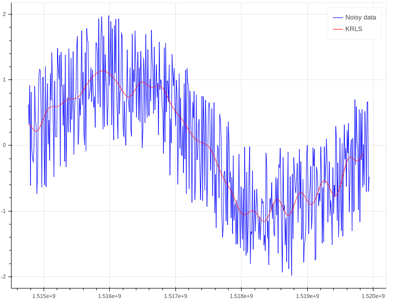
The following code computes a interpolated time-series for the predictor for the entire range of the underlying data to demonstrate how to compute interpolations and also that interpolations can be computed outside the trained range.
predict_dt = deltaminutes(30)  # time-step in predicted time-series
predict_period = UtcPeriod(t0, utc.time(2018, 3, 1))  # period to predict for

# create a time-series for prediction
krls_predict_ts = TimeSeries(
    r'shyft://data/sine?container=krls'
    f'&dt={predict_dt}'  # if unspecified: defaults to 3600 (1 hour)
)

# predict a time-series
tsv = TsVector()
tsv.append(krls_predict_ts)
# -----
tsv = client.evaluate(tsv, predict_period)

# plot with bokeh
fig = figure(width=800)
fig.line(time_axis_extract_time_points(data_ts.get_time_axis())[:-1], data_ts.values, legend_label='Noisy data', color='blue')
fig.line(time_axis_extract_time_points(tsv[0].get_time_axis())[:-1], tsv[0].values, legend_label='KRLS', color='red')
show(fig)
3. Update the trained period
To update the period a predictor is trained on we write to the series with a time-series spanning the period we want.
To not rewrite the entire predictor remember to call DtsClient.store with overwrite_on_write=False!
And unless you also specify allow_period_gap=true the periods need to overlap or be consecutive.
Also note that you currently cannot replace only a smallportion of the data the predictor have trained on. If you need to retrain you have to delete the predictor and start over again.
The next code cell demonstrates that writing to the series again with overwrite_on_write=False argument to the DTS client store updates the saved predictor.
# use the full time-axis for the data range this time

# create the time-series to register a krls predictor
krls_register_ts = TimeSeries(
    r'shyft://data/sine?container=krls',
    # A limitation of the krls server/client is that we need to send a time-series with data.
    # Currently the period of this time-series is used to specify the period we train KRLS on.
    TimeSeries(ta, 0., POINT_INSTANT_VALUE)
)

# register and train predictor initially
tsv = TsVector()
tsv.append(krls_register_ts)
# -----
client.store_ts(tsv, overwrite_on_write=False)
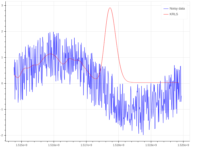
4. Repredict
Recompute to see that the trained period have updated.
predict_dt = deltaminutes(30)  # time-step in predicted time-series
predict_period = UtcPeriod(t0, utc.time(2018, 3, 1))  # period to predict for

# create a time-series for prediction
krls_predict_ts = TimeSeries(
    r'shyft://data/sine?container=krls'
    f'&dt={predict_dt}'  # if unspecified: defaults to 3600 (1 hour)
)

# predict a time-series
tsv = TsVector()
tsv.append(krls_predict_ts)
# -----
tsv = client.evaluate(tsv, predict_period)

# plot with bokeh
fig = figure(width=800)
fig.line(time_axis_extract_time_points(data_ts.get_time_axis())[:-1], data_ts.values, legend_label='Noisy data', color='blue')
fig.line(time_axis_extract_time_points(tsv[0].get_time_axis())[:-1], tsv[0].values, legend_label='KRLS', color='red')
show(fig)