Kalman filtering on gridded data
Setup environment for tutorials
This notebook gives an example of Met.no data post-processing to correct temperature forecasts based on comparison to observations. The following steps are described:
Loading required python modules and setting path to Shyft installation
Setup steps is about creating synthetic data, and backtesting those so that we have a known forecast that gives a certain response at the four observation points
Generate synthetic data for temperature observation time-series
Transform observations from set to grid (Kriging)
Create 3 forecasts sets for the 1x1 km grid
grid-pp steps is about orchestrating a grid-pp algorithm given our syntethic data from above
Transform forecasts from grid to observation points (IDW)
Calculate the bias time-series using Kalman filter on the difference of observation and forecast set at the observation points
Transform bias from set to grid (Kriging) and apply bias to the grid forecast
Final steps to plot and test the results from the grid-pp steps
Transform corrected forecasts grid to the observation points (IDW)
Plot the results and bias
1. Loading required python modules and setting path to Shyft installation
# first you should import the third-party python modules which you'll use later on
# the first line enables that figures are shown inline, directly in the notebook
%matplotlib inline
import os
from os import path
import sys
from matplotlib import pyplot as plt
# once the shyft_path is set correctly, you should be able to import shyft modules
import shyft
from shyft.hydrology import shyftdata_dir
import shyft.hydrology as api
import shyft.time_series as sts

# if you have problems here, it may be related to having your LD_LIBRARY_PATH
# pointing to the appropriate libboost_python libraries (.so files)
from shyft.hydrology.repository.default_state_repository import DefaultStateRepository
from shyft.hydrology.orchestration.configuration import yaml_configs
from shyft.hydrology.orchestration.simulators.config_simulator import ConfigSimulator
from shyft.time_series import Calendar
from shyft.time_series import deltahours
from shyft.time_series import TimeAxis
from shyft.time_series import TimeSeries
from shyft.time_series import time_shift
from shyft.hydrology import TemperatureSource
from shyft.hydrology import TemperatureSourceVector
from shyft.hydrology import GeoPoint
from shyft.hydrology import GeoPointVector
from shyft.hydrology import bayesian_kriging_temperature
from shyft.hydrology import BTKParameter
from shyft.hydrology import idw_temperature
from shyft.hydrology import IDWTemperatureParameter
from shyft.hydrology import KalmanFilter
from shyft.hydrology import KalmanState
from shyft.hydrology import KalmanBiasPredictor
from shyft.time_series import create_periodic_pattern_ts
from shyft.time_series import POINT_AVERAGE_VALUE as stair_case
# now you can access the api of shyft with tab completion and help, try this:

#help(api.GeoPoint) # remove the hashtag and run the cell to print the documentation of the api.GeoPoint class
#api. # remove the hashtag, set the pointer behind the dot and use
    # tab completion to see the available attributes of the shyft api
Setup: 1. Generate synthetic data for temperature observation time-series
# Create time-axis for our syntethic sample
utc = Calendar() # provide conversion and math for utc time-zone
t0 = utc.time(2016, 1, 1)
dt = deltahours(1)
n = 24*3 # 3 days length
#ta = TimeAxisFixedDeltaT(t0, dt, n)
ta = TimeAxis(t0, dt, n) # same as ta, but needed for now(we work on aligning them)

# 1. Create the terrain based geo-points for the 1x1km grid and the observations

# a. Create the grid, based on a syntethic terrain model
# specification of 1 x 1 km
grid_1x1 = GeoPointVector()
for x in range(10):
    for y in range(10):
        grid_1x1.append(GeoPoint(x*1000, y*1000, (x+y)*50)) # z from 0 to 1000 m

# b. Create the observation points, for metered temperature
# reasonable withing that grid_1x1, and with elevation z
# that corresponds approximately to the position
obs_points = GeoPointVector()
obs_points.append(GeoPoint( 100, 100, 10))  # observation point at the lowest part
obs_points.append(GeoPoint(5100, 100, 270 )) # halfway out in x-direction @ 270 masl
obs_points.append(GeoPoint( 100, 5100, 250)) # halfway out in y-direction @ 250 masl
obs_points.append(GeoPoint(10100,10100, 1080 )) # x-y at max, so @1080 masl

# 2. Create time-series having a constant temperature of 15 degC
#    and add them to the syntetic observation set
#    make sure there is some reality, like temperature gradient etc.
ts = TimeSeries(ta, fill_value=20.0,point_fx=stair_case)  # 20 degC at z_t= 0 meter above sea-level
# assume set temp.gradient to -0.6 degC/100m, and estimate the other values accordingly
tgrad = -0.6/100.0  # in our case in units of degC/m
z_t = 0 # meter above sea-level

# Create a TemperatureSourceVector to hold the set of observation time-series
constant_bias=[-1.0,-0.6,0.7,+1.0]
obs_set = TemperatureSourceVector()
obs_set_w_bias = TemperatureSourceVector()
for geo_point,bias in zip(obs_points,constant_bias):
    temp_at_site =  ts + tgrad*(geo_point.z-z_t)
    obs_set.append(TemperatureSource(geo_point,temp_at_site))
    obs_set_w_bias.append(TemperatureSource(geo_point,temp_at_site + bias))
Setup 2. Transform observation with bias to grid using kriging
# Generate the observation grid by kriging the observations out to 1x1km grid
# first create idw and kriging parameters that we will utilize in the next steps
# kriging parameters
btk_params = BTKParameter()  # we could tune parameters here if needed
# idw parameters,somewhat adapted to the fact that we
#  know we interpolate from a grid, with a lot of neigbours around
idw_params = IDWTemperatureParameter() # here we could tune the paramete if needed
idw_params.max_distance = 20*1000.0 # max at 10 km because we search for max-gradients
idw_params.max_members = 20 # for grid, this include all possible close neighbors
idw_params.gradient_by_equation = True # resolve horisontal component out
# now use kriging for our 'syntethic' observations with bias
obs_grid = bayesian_kriging_temperature(obs_set_w_bias,grid_1x1,ta.fixed_dt,btk_params)


# if we idw/btk back to the sites, we should have something that equals the with_bias:
# we should get close to zero differences in this to-grid-and-back operation
back_test = idw_temperature(obs_grid, obs_points, ta.fixed_dt, idw_params)  # note the ta.fixed_dt here!
for bt,wb in zip(back_test,obs_set_w_bias):
    print("IDW Diff {} : {} ".format(bt.mid_point(),abs((bt.ts-wb.ts).values).max()))

#back_test = bayesian_kriging_temperature(obs_grid, obs_points, ta, btk_params)
#for bt,wb in zip(back_test,obs_set_w_bias):
#    print("BTK Diff {} : {} ".format(bt.mid_point(),abs((bt.ts-wb.ts).values).max()))
Output:
IDW Diff GeoPoint(100.0,100.0,10.0) : 0.0268954741303169
IDW Diff GeoPoint(5100.0,100.0,270.0) : 0.03278720737025864
IDW Diff GeoPoint(100.0,5100.0,250.0) : 0.056529126054066126
IDW Diff GeoPoint(10100.0,10100.0,1080.0) : 0.004978394987212198
Setup 3. Create 3 forecasts sets for the 1x1 km grid
# Create a forecast grid by copying the obs_grid time-series
# since we know that idw of them to obs_points will give approx.
#  the obs_set_w_bias time-series
#  for the simplicity, we assume the same forecast for all 3 days

fc_grid = TemperatureSourceVector()
fc_grid_1_day_back = TemperatureSourceVector() # this is previous day
fc_grid_2_day_back = TemperatureSourceVector()  # this is fc two days ago
one_day_back_dt = deltahours(-24)
two_days_back_dt = deltahours(-24*2)
noise_bias = [0.0 for i in range(len(obs_grid))] # we could generate white noise ts into these to test kalman
for fc,bias in zip(obs_grid,noise_bias):
    fc_grid.append(TemperatureSource(fc.mid_point(),fc.ts + bias ))
    fc_grid_1_day_back.append(
        TemperatureSource(
                fc.mid_point(),
                time_shift(fc.ts + bias, one_day_back_dt) #time-shift the signal back
            )
        )
    fc_grid_2_day_back.append(
        TemperatureSource(
                fc.mid_point(),
                time_shift(fc.ts + bias, two_days_back_dt)
            )
        )

grid_forecasts = [fc_grid_2_day_back, fc_grid_1_day_back, fc_grid ]
grid-pp: 1. Transform forecasts from grid to observation points (IDW)
# Now we have 3 simulated forecasts at a 1x1 km grid
# fc_grid, fc_grid_1_day_back, fc_grid_2_day_back
# we start to do the grid pp algorithm stuff
# - we know the our forecasts have some degC. bias, and we would hope that
#   the kalman filter 'learns' the offset
# as a first step we project the grid_forecasts to the observation points
# making a list of historical forecasts at each observation point.

fc_at_observation_points = [idw_temperature(fc, obs_points, ta.fixed_dt, idw_params)\
                            for fc in grid_forecasts]
historical_forecasts = []
for i in range(len(obs_points)):  # correlate obs.point and fc using common i
    fc_list = TemperatureSourceVector()  # the kalman bias predictor below accepts TsVector of forecasts
    for fc in fc_at_observation_points:
        fc_list.append(fc[i]) # pick out the fc_ts only, for the i'th observation point
        #print("{} adding fc pt {} t0={}".format(i,fc[i].mid_point(),utc.to_string(fc[i].ts.time(0))))
    historical_forecasts.append(fc_list)
# historical_forecasts  now cntains 3 forecasts for each observation point
grid-pp: 2. Calculate the bias time-series using Kalman filter on the observation set
# Create a TemperatureSourceVector to hold the set of bias time-series
bias_set = TemperatureSourceVector()

# Create the Kalman filter having 8 samples spaced every 3 hours to represent a daily periodic pattern

kalman_dt_hours = 3
kalman_dt =deltahours(kalman_dt_hours)
kta = TimeAxis(t0, kalman_dt, int(24//kalman_dt_hours))

# Calculate the coefficients of Kalman filter and
# Create bias time-series based on the daily periodic pattern
for i in range(len(obs_set)):
    kf = KalmanFilter() # each observation location do have it's own kf &predictor
    kbp = KalmanBiasPredictor(kf)
    #print("Diffs for obs", i)
    #for fc in historical_forecasts[i]:
    #    print((fc.ts-obs_set[i].ts).values)
    kbp.update_with_forecast(historical_forecasts[i], obs_set[i].ts, kta)
    pattern = KalmanState.get_x(kbp.state)
    #print(pattern)
    bias_ts = create_periodic_pattern_ts(pattern, kalman_dt, ta.time(0), ta)
    bias_set.append(TemperatureSource(obs_set[i].mid_point(), bias_ts))
grid-pp: 3. Spread the bias at observation points out to the grid using kriging
# Generate the bias grid by kriging the bias out on the 1x1km grid
btk_params = BTKParameter()
btk_bias_params = BTKParameter(temperature_gradient=-0.6, temperature_gradient_sd=0.25, sill=25.0, nugget=0.5, range=5000.0, zscale=20.0)
bias_grid =  bayesian_kriging_temperature(bias_set, grid_1x1, ta.fixed_dt, btk_bias_params)
# Correct forecasts by applying bias time-series on the grid
fc_grid_improved = TemperatureSourceVector()
for i in range(len(fc_grid)):
    fc_grid_improved.append(
        TemperatureSource(
            fc_grid[i].mid_point(),
            fc_grid[i].ts - bias_grid[i].ts # By convention, sub bias time-series(hmm..)
        )
    )
# Check the first value of the time-series. It should be around 15
tx =ta.time(0)
print("Comparison original synthetic grid cell [0]\n\t at the lower left corner,\n\t at t {}\n\toriginal grid: {}\n\timproved grid: {}\n\t vs bias grid: {}\n\t nearest obs: {}"
    .format(utc.to_string(tx),
            fc_grid[0].ts(tx),
            fc_grid_improved[0].ts(tx),
            bias_grid[0].ts(tx),
            obs_set[0].ts(tx)
            )
    )
Output:
Comparison original synthetic grid cell [0]
     at the lower left corner,
     at t 2016-01-01T00:00:00Z
    original grid: 18.985602994491913
    improved grid: 19.740020177551433
     vs bias grid: -0.7544171830595209
     nearest obs: 19.94
Presentation&Test: 8. Finally, Transform corrected forecasts from grid to observation points to see if we did reach the goal of adjusting the forecast (IDW)
# Generate the corrected forecast set by Krieging transform of temperature model
fc_at_observations_improved = idw_temperature(fc_grid_improved, obs_points, ta.fixed_dt, idw_params)
fc_at_observations_raw =idw_temperature(fc_grid, obs_points, ta.fixed_dt, idw_params)
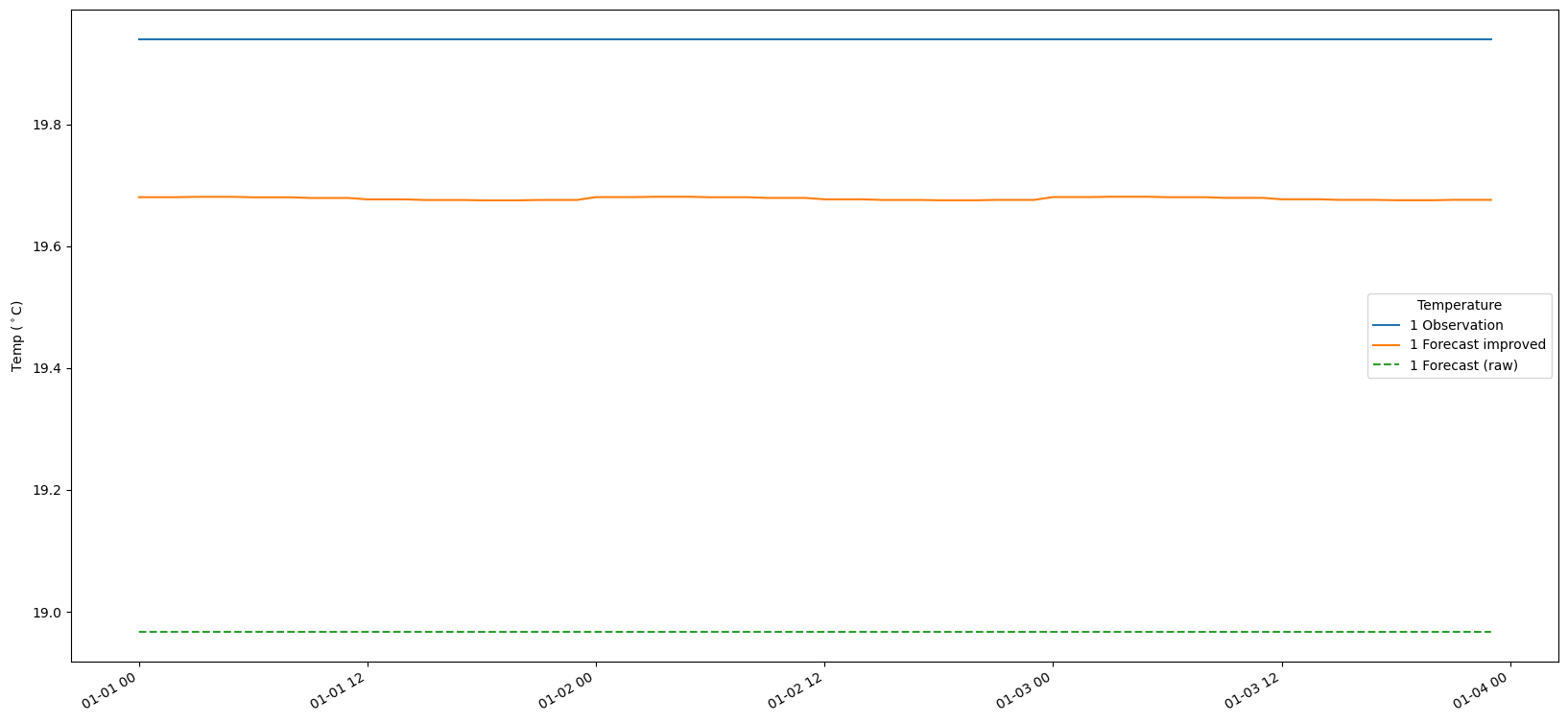
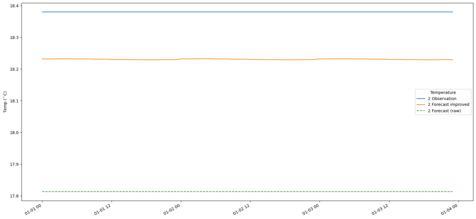
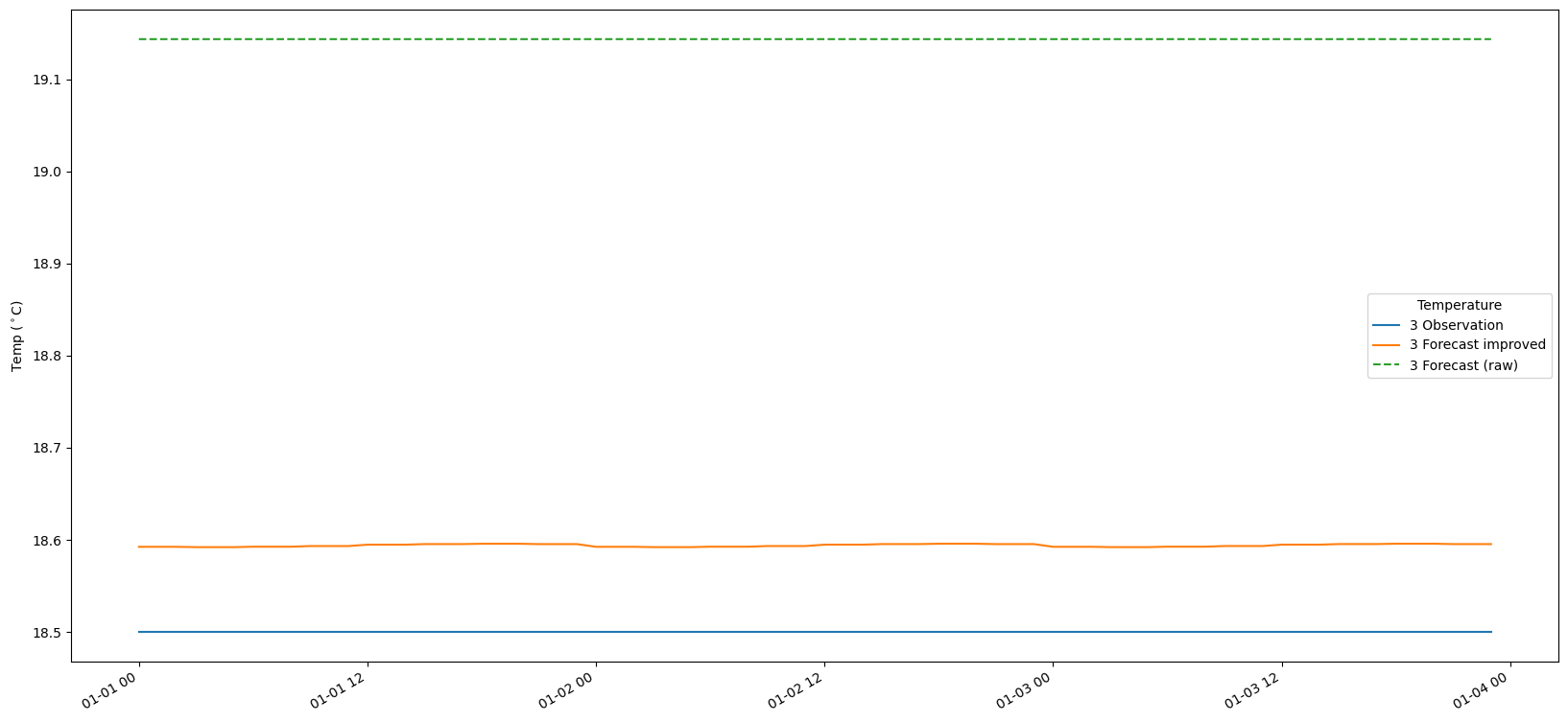
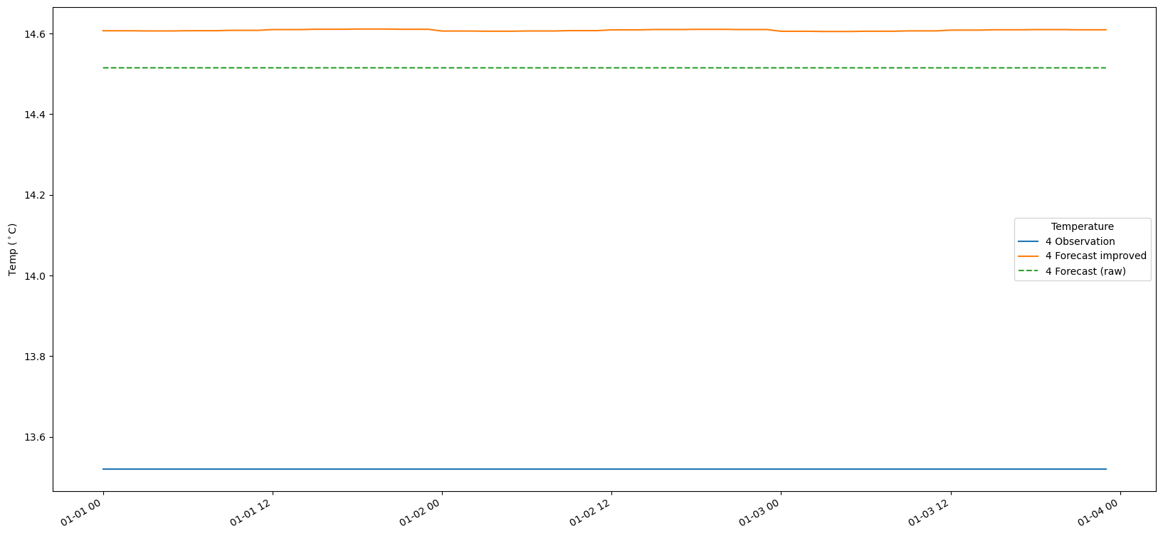
9. Plot the results
# Make a time-series plot of temperature sets
for i in range(len(bias_set)):
    fig, ax = plt.subplots(figsize=(20, 10))
    timestamps = [datetime.datetime.utcfromtimestamp(p) for p in obs_set[i].ts.time_axis.time_points]
    ax.plot(timestamps[:-1], obs_set[i].ts.values, label = str(i+1) + ' Observation')
    ax.plot(timestamps[:-1], fc_at_observations_improved[i].ts.values, label = str(i+1) + ' Forecast improved')
    ax.plot(timestamps[:-1], fc_at_observations_raw[i].ts.values,linestyle='--', label = str(i+1) + ' Forecast (raw)')
    #ax.plot(timestamps, bias_set[i].ts.values, label = str(i+1) + ' Bias')
    fig.autofmt_xdate()
    ax.legend(title='Temperature')
    ax.set_ylabel('Temp ($^\circ$C)')
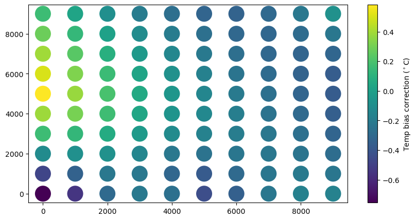
# Make a scatter plot of grid temperature forecasts at ts.value(0)
x = [fc.mid_point().x for fc in bias_grid]
y = [fc.mid_point().y for fc in bias_grid]
fig, ax = plt.subplots(figsize=(10, 5))
temps = np.array([bias.ts.value(0) for bias in bias_grid])
plot = ax.scatter(x, y, c=temps, marker='o', s=500, lw=0)
plt.colorbar(plot).set_label('Temp bias correction ($^\circ$C)')