Single method point simulation
Setup environment for tutorials
Introduction
There are several cases when one may be interested to evaluate a method as an independent entity from a full simulation domain. One may be interested in exploring a snow melt routine, or an evapotranspiration calculation and comparing it with local point observations. Or, you may be interested to explore a method and evaluate the parameter sensitivity.
While Shyft provides a toolbox for running distributed hydrologic simulations, we recognize the need for point-based simulations as well. We have provided several different mechanisms for running the models. The main concept to be aware of is that while we demonstrate and build on the use of a ‘configuration’, nearly all simulation functionality is also accessible with pure python. It is recommended, if you intend to use Shyft for any kind of hydrologic exploration, to become familiar with the API functionality.
In this python tutorial, you will learn how to use the Shyft API to directly access single methods used in model stacks. You will learn how to run them without running a complete model stack and without using any ‘configuration’ layer or simulation. This functionality allows one to explore certain model routines as a point model (e.g. for comparison of model results with point observations), conducting sensitivity studies, and investigating the details of a certain routine.
To achive this, we will:
Create a synthetic data set which we will use to run the model
Convert the input data to shyft-conform data-types by using Shyft’s API functionality
Run a certain routine using the Shyft API (we will use the HBV snow routine as an example)
Change the default parameters and initial state
The Shyft Environment
# Pure python modules and jupyter notebook functionality
# first you should import the third-party python modules which you'll use later on
# the first line enables that figures are shown inline, directly in the notebook
%matplotlib inline
import os
from os import path
import sys
import numpy as np
from matplotlib import pyplot as plt
Set shyft-data path:
# try to auto-configure the path, -will work in all cases where doc and data
# are checked out at same level
from shyft.hydrology import shyftdata_dir

shyft_data_path = os.path.abspath("/workspaces/shyft-data/")
if path.exists(shyft_data_path) and 'SHYFT_DATA' not in os.environ:
    os.environ['SHYFT_DATA']=shyft_data_path
# once the shyft_path is set correctly, you should be able to import shyft modules, e.g. the shyft API
from shyft.hydrology import HbvSnowCalculator,HbvSnowParameter,HbvSnowState,HbvSnowResponse
from shyft.time_series import (Calendar,time,UtcPeriod,deltahours,
                            TimeAxis,TimeSeries,DoubleVector,
                            point_interpretation_policy)
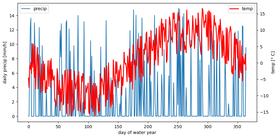
1. Synthetic forcing data set
n = 365 # nr of time steps: 1 year, daily data
precip_bool = [0 if r <0.7 else 1 for r in np.random.rand(n)]
precip = [i*j*15 for i,j in zip(np.random.rand(n),precip_bool)] # precip [mm/day]
temp_noise = (np.random.rand(n)-0.5) * 15
temp = 10 * np.sin(-np.arange(n)*2*np.pi/n) + temp_noise # temperatur [deg C]
day = np.arange(n) # day of water year
# Let's have a look to the synthetic forcing data by plotting it
fig, ax1 = plt.subplots(figsize=(10,5))
ax2 = ax1.twinx()
ax1.plot(day,precip, label='precip')
ax2.plot(day, temp, c='r', lw=2, label='temp')
ax1.set_ylabel('daily precip [mm/h]')
ax2.set_ylabel('temp [$°$ C]')
ax1.set_xlabel('day of water year')
ax1.legend(loc=2); ax2.legend(loc=1)
2. Convert input data to shyft-conform data-types by using api functionality
# Every routine (e.g. for computing the snowpack, evapotranspiration, discharge response, ...)
# has a "Calculator" class, here shown for the HbvSnow routine:
type(HbvSnowCalculator)
# Let's print some information about the calculator class
help(HbvSnowCalculator)
Output:
Docstring:
Generalized quantile based HBV Snow model method

This algorithm uses arbitrary quartiles to model snow. No checks are performed to assert valid input.
The starting points of the quantiles have to partition the unity,
include the end points 0 and 1 and must be given in ascending order.
Init docstring:
__init__( (HbvSnowCalculator)arg1, (HbvSnowParameter)parameter) -> None :
    creates a calculator with given parameter
File:           /usr/local/lib64/python3.11/site-packages/shyft/hydrology/_api.so
Type:           class
Subclasses:
Using tab-completion, we can check out the methods the calculator-class is providing Try it out by uncommenting the line below and press the “tab” key on your keyboard:
api.HbvSnowCalculator.
Obviously, there is a method called “step”. This method can be used to do the time stepping. E.g. if we have a certain model state s0 at time t0, the step function calculates the model state s1 at time t0+dt, where dt is the time step in seconds.
The Calculator classes of all routines have a similar method. In most cases this method is called “step”, such as here. Let’s check out the details of the “step” method in more detail:
help(HbvSnowCalculator.step)
Output:
Docstring:
step( (HbvSnowCalculator)self, (HbvSnowState)state, (HbvSnowResponse)response, (time)t0, (time)t1, (float)precipitation, (float)temperature) -> None :
    steps the model forward from t0 to t1, updating state and response

Type:      function
The docstring of this method tells us, that the follwoing arguments are required to step forward by one time step dt:
model state of type “HbvSnowState”
model response of type “HbvSnowResponse”
start time t0 of type “int”
end time t1 of type “int”
model parameters of type “HbvSnowParameter”
precipitation input of type “float”
temperature input of type “float”
If we can provide the above listed input, we can step the model forward.
# The shyft api supports quite some functionality for time and time series handling
# lets assume that the synthetic data is daily data, starting at October 1st, 2016
utc = Calendar() # provides shyft build-in functionality for date/time handling
t_start = utc.time(2016, 10, 1) # starting at the beginning of the water year 2017
dt = deltahours(24) # returns daily timestep in seconds
# Let's now create Shyft time series from the supplied lists of precipitation and temperature.
# First, we need a time axis, which is defined by a starting time, a time step and the number of time steps.
ta = TimeAxis(t_start, dt, n)
# We now can transform our python-type lists to Shyft type time series.
# To get more information about the time series, have a look into the
# "ts-convolve" and the "partition_by_and_percentiles" notebooks.

# First, we convert the lists to shyft internal vectors of double values:
temp_dv = DoubleVector(temp) #.from_numpy(temp)
precip_dv = DoubleVector(precip) #.from_numpy(precip)

# The TimeSeries class has some powerfull funcionality (however, this is not subject of matter in here).
# For this reason, one needs to specify how the input data can be interpreted:
# - as instant point values at the time given (e.g. such as most observed temperatures), or
# - as average value of the period (e.g. such as most observed precipitation)
# This distinction can be specified by passing the respective "point_interpretation_policy",
# provided by the API:
instant = point_interpretation_policy.POINT_INSTANT_VALUE
average = point_interpretation_policy.POINT_AVERAGE_VALUE

# Finally, we create shyft time-series as follows:
# (Note: This step is not necessarily required to run the single methods.
#  We could also just work with the double vector objects and the time axis)
temp_ts = TimeSeries(ta, temp_dv, point_fx=instant)
precip_ts = TimeSeries(ta, precip_dv, point_fx=average)
3. Run a method using the Shyft API
To run the routine now step by step, we first need to instanciate an instance of the calculator object. To instanciete the calculator class we need to provide the starting state of our model (the values of all state variables at time t0) and the model parameters at time t0 as arguments. The model state will later be updated by the routine. If we would like to, we can update the model parameters as well. More to this further down.
parameter = HbvSnowParameter()
state = HbvSnowState()
state.distribute(parameter)  # the state also contains a snow distribution, these needs to match parameter
response = HbvSnowResponse()

calculator = HbvSnowCalculator(parameter)
# Let's first have a look to the starting state of our model: you can use tab completing
# to investigate the state-variables of the HbvSnow algorithm (try out!)
state.sca

# output: 0
# we now can simply run the routine step by step:
try:
    del outflow
except:
    pass
for i in range(n):
    P = precip_ts.v[i]
    T = temp_ts.v[i]
    t0 = t_start + i*dt
    t1 = t0 + dt
    calculator.step(state, response, t0, t1, P, T)
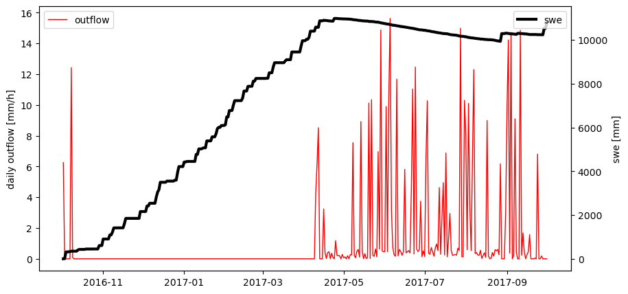
However, so far we didn’t get any information about state and response variables from the model. Let’s repeat the run - this time collecting the state and response variables. (Note: Collecting state and response variables is done by so called “collectors” when running a model stack available in shyft, e.g. the pt_gs_k stack. Here, we simply append the model state and response of each time step to shyft’s double vectors.)
swe = DoubleVector() # double vector to collect snow water equivalent, a state variable of HbvSnow; the double vector is empty so far
outflow = DoubleVector() # double vector to collect outflow from the snow pack, a response variable of HbvSnow.
state = HbvSnowState() # reset the model state to default
state.distribute(parameter) # recall, hbv.snow state have a distribution in bins, number of bins must also initialize
for i in range(n):
    P = precip_ts.v[i]
    T = temp_ts.v[i]
    t0 = t_start + i*dt
    t1 = t0 + dt
    calculator.step(state, response, t0, t1, P, T)
    swe.append(state.swe) # appending the current model state to the double vector
    outflow.append(response.outflow) # appending the current model respnse to the double vector
# Let's also create a time axis suiting to the collected state and response:
# (Note: the first collection of a state and response refers to t_start+dt)
ta_state = TimeAxis(t_start+dt, dt, n-1)
# Using this time axis, we can create a list of datetime objects which will use during plotting
dates = [datetime.datetime.utcfromtimestamp(t) for t in ta_state.time_points]
print(len(outflow))
# Let's plot the data we received from HbvSnow
fig, ax1 = plt.subplots(figsize=(10,5))
ax2 = ax1.twinx()
ax1.plot(dates, outflow, c='r', lw=1, label='outflow')
ax2.plot(dates, swe, c='k', lw=3, label='swe')
ax1.set_ylabel('daily outflow [mm/h]')
ax2.set_ylabel('swe [mm]')
ax1.legend(loc=2); ax2.legend(loc=1)
4. Changing parameters and initial state
So far we ran the routine only with the default parameters and state. Shyft provides the functionality to set starting state and parameters on the fly as needed.
Use tab completion to investigate on which parameters HbvSnow depends
Use the ‘help’ functionality to get information about a certain parameter, e.g. cx
help(parameter.cx)
Output:
Type:        property
String form: <property object at 0x7f39d30a8d60>
Docstring:   float: temperature index, i.e., melt = cx(t - ts) in mm per degree C
Let’s look at the default value of the parameter cx:
print(parameter.cx)

# output: 1.0
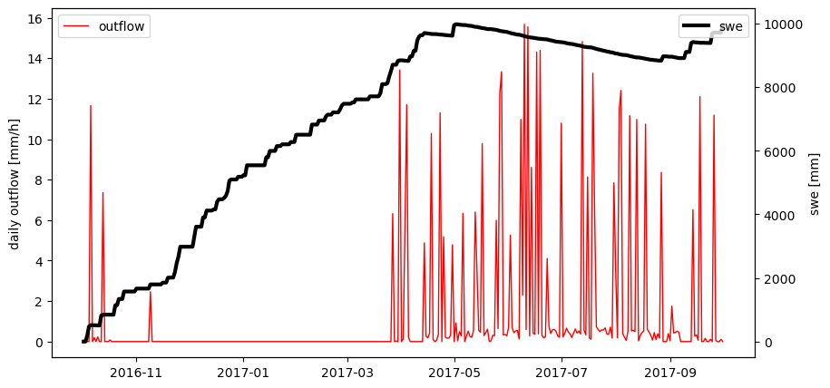
Lets now set a parameter to a new value and rerun HbvSnow and replot the outcome
parameter.cx = 2.0

swe = DoubleVector()
outflow = DoubleVector()
state = HbvSnowState() # reset the model state to default
state.distribute(parameter) # again, the snow.distribution needs to match the parameter,
calculator = HbvSnowCalculator(parameter)
for i in range(n):
    P = precip_ts.v[i]
    T = temp_ts.v[i]
    t0 = t_start + i*dt
    t1 = t0 + dt
    calculator.step(state, response, t0, t1, P, T)
    swe.append(state.swe) # appending the current model state to the double vector
    outflow.append(response.outflow) # appending the current model respnse to the double vector
# Let's plot the data we received from HbvSnow
fig, ax1 = plt.subplots(figsize=(10,5))
ax2 = ax1.twinx()
ax1.plot(dates, outflow, c='r', lw=1, label='outflow')
ax2.plot(dates, swe, c='k', lw=3, label='swe')
ax1.set_ylabel('daily outflow [mm/h]')
ax2.set_ylabel('swe [mm]')
ax1.legend(loc=2); ax2.legend(loc=1)
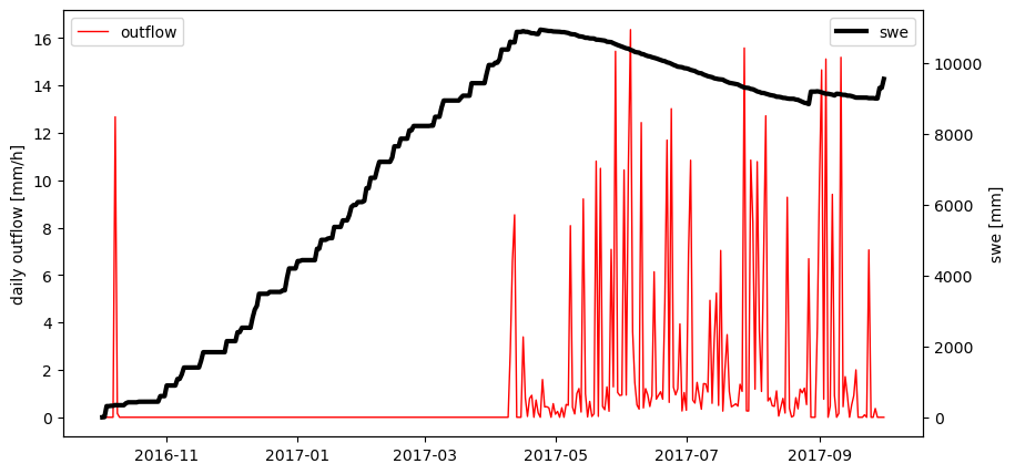
To complete the training, let’s also set a different starting state, e.g. an already existing snow pack:
swe = DoubleVector()
outflow = DoubleVector()
state = HbvSnowState() # reset the model state to default
state.distribute(parameter) # recall, snow state keeps distribution, an unknown number of bins until told by distribute
parameter = HbvSnowParameter() # reset the model parameters to default
# setting a certain starting state
state.sca = 1.0
state.swe = 150.0
# rerun the model
calculator = HbvSnowCalculator(parameter)
for i in range(n):
    P = precip_ts.v[i]
    T = temp_ts.v[i]
    t0 = t_start + i*dt
    t1 = t0 + dt
    calculator.step(state, response, t0, t1, P, T)
    swe.append(state.swe) # appending the current model state to the double vector
    outflow.append(response.outflow) # appending the current model respnse to the double vector
# Let's plot the data we received from HbvSnow
fig, ax1 = plt.subplots(figsize=(10,5))
ax2 = ax1.twinx()
ax1.plot(dates, outflow, c='r', lw=1, label='outflow')
ax2.plot(dates, swe, c='k', lw=3, label='swe')
ax1.set_ylabel('daily outflow [mm/h]')
ax2.set_ylabel('swe [mm]')
ax1.legend(loc=2); ax2.legend(loc=1)