Penman-Monteith Single Method Verification

Setup environment for tutorials

The purpose of this notebook is to verify that Shyft implementation of Full Penman-Monteith (FPM) and Standardized Penman-Monteith (SPM) equations match reference data provided in ASCE-EWRI, Appendix C.

ref.: The ASCE Standardized Reference Evapotranspiration Equation,
    Environmental and Water Resources Institute (EWRI) of the American Society of Civil Engineers Task Committee
    on Standardization of Reference Evapotranspiration Calculation, ASCE, Washington, DC, 2005

First we will import all necessary content

import os
import sys
import math
from matplotlib import pyplot as plt
from datetime import datetime
import shyft.hydrology as api
from shyft.time_series import (Calendar,deltahours,UtcPeriod,TimeSeries,TimeAxis,DoubleVector,point_interpretation_policy)

The ASCE-EWRI Appendix C provides verification reference data for
daily time steps: 10 days in July, 2000.
hourly time steps: 31-hour period from 16.00 on July 1 to 22.00 on July 2, 2000
Station: Greeley, Colorado
Latitude: 40.41 degrees N,
Longitude: 104.78 degrees W,
Elevation: 1462.4 m,
Anemometer height: 3 m,
Height of temperature/RH meas.: 1.68 m,
Type of surface: irrigated grass,
Height veg.: 0.12 m (short crop) or 0.5 (tall crop)

24-hour time-step

utc = Calendar() # provides shyft build-in functionality for date/time handling
# Single method test based on ASCE-EWRI Appendix C, daily time-step
# Station data: Greeley, Colorado
# Location:
latitude = 40.41
longitude = 104.78
elevation = 1462.4
# Height of measurements
height_ws = 3 # height of anemometer
height_t = 1.68 # height of air temperature and rhumidity measurements
# Vegetation info
surface_type = "irrigated grass"
height_veg = 0.12 #vegetation height, short crop
# height_veg = 0.5 #vegetation height, tall crop
# values for stomatal resistance were recalculated based on the info about bulk surface resistances and
# equations B.3-B.6
rl = 100.8 #stomatal resistance, short crop
if height_veg>0.12:
    rl = 100.35 # tall crop
# Some calculated parameters from reference
atm_pres_mean = 85.17 #[kPa]
psychrom_const = 0.0566
windspeed_adj = 0.921
# Data for radiation model, which can be also added into calculations, so there is an option to run either with
# measured radiation or with simulated one
lat_rad = latitude*math.pi/180
slope_deg = 0.0
aspect_deg = 0.0

Let’s create TimeAxis first (I assume that user already familiarizes himself with shyft timeseries concepts)

n = 10 # nr of time steps: 1 year, daily data
t_start = utc.time(2000, 7, 1) # starting point: 1-07-2000
t_end = utc.time(2000, 7, 10, 23,0,0,0) # end point: 10-07-2000
dtdays = deltahours(24) # returns daily timestep in seconds

# First, we need a time axis, which is defined by a starting time, a time step and the number of time steps.
tadays = TimeAxis(t_start, dtdays, n) # days
period = UtcPeriod(t_start,t_end)
# print(len(tadays))

The reference provides the following weather data:

# Data from weather station
ws_Tmax = [32.4, 33.6, 32.6, 33.8, 32.7, 36.3, 35.5, 34.4, 32.7, 32.7] # Max air temperature, [degC]
ws_Tmin = [10.9, 12.2, 14.8, 11.8, 15.9, 15.8, 16.7, 18.3, 15.1, 15.7] # Min air temperature, [degC]
ws_ea = [1.27, 1.19, 1.40, 1.18, 1.59, 1.58, 1.13, 1.38, 1.38, 1.59]  # actual vapor pressure, [kPa]
ws_Rs = [22.4, 26.8, 23.3, 29.0, 27.9, 29.2, 23.2, 22.1, 26.5, 27.7] # Incoming shortwave radiation, [Mj/m^2/day]
ws_windspeed = [1.94, 2.14, 2.06, 1.97, 2.98, 2.37, 2.43, 1.95, 1.75, 2.31] # Windspeed, [m/s]

# Results from reference:
ET_os_daily = [5.71, 6.71, 5.98, 6.86, 7.03, 7.50, 7.03, 6.16, 6.20, 6.61] # short crop evapotranspiration
ET_rs_daily = [7.34, 8.68, 7.65, 8.73, 9.07, 9.60, 9.56, 7.99, 7.68, 8.28] # tall crop evapotranspiration
rso_d_ref = [32.43, 32.39, 32.36, 32.32, 32.27, 32.23, 32.18, 32.13, 32.08, 32.02] # simulated insolation
rnet_d_ref = [13.31, 15.20, 13.78, 16.19, 16.33, 16.83, 13.15, 13.00, 15.27, 16.15] # net radiation simulated

# conversions
c_MJm2d2Wm2 = 0.086400
c_MJm2h2Wm2 = 0.0036

Our implementation of Penman-Monteith requires Relative Humidity as imput, so we recalculate from weather data:

#recalculated inputs
ws_Tmean = []
ws_rhmean = []
ws_svp_tmean = []

for i in range(len(ws_Tmax)):
    ws_Tmean.append((ws_Tmax[i]+ws_Tmin[i])*0.5)

for i in range(len(ws_Tmax)):
    ws_svp_tmean.append(0.6108 * math.exp(17.27 * ws_Tmean[i] / (ws_Tmean[i] + 237.3)))

for i in range(len(ws_Tmax)):
    ws_rhmean.append(ws_ea[i]*100/ws_svp_tmean[i])

From the provided data we create Timeseries, which will be used as an input to our method

# First, we convert the lists to shyft internal vectors of double values:
tempmax_dv = DoubleVector.from_numpy(ws_Tmax)
tempmin_dv = DoubleVector.from_numpy(ws_Tmin)
ea_dv = DoubleVector.from_numpy(ws_ea)
rs_dv = DoubleVector.from_numpy(ws_Rs)
windspeed_dv = DoubleVector.from_numpy(ws_windspeed)

tempmean_dv = DoubleVector.from_numpy(ws_Tmean)
rhmean_dv = DoubleVector.from_numpy(ws_rhmean)

# The TimeSeries class has some powerfull funcionality (however, this is not subject of matter in here).
# For this reason, one needs to specify how the input data can be interpreted:
# - as instant point values at the time given (e.g. such as most observed temperatures), or
# - as average value of the period (e.g. such as most observed precipitation)
# This distinction can be specified by passing the respective "point_interpretation_policy",
# provided by the API:
instant = point_interpretation_policy.POINT_INSTANT_VALUE
average = point_interpretation_policy.POINT_AVERAGE_VALUE

# Finally, we create shyft time-series as follows:
# (Note: This step is not necessarily required to run the single methods.
#  We could also just work with the double vector objects and the time axis)
tempmax_ts = TimeSeries(tadays, tempmax_dv, point_fx=instant)
tempmin_ts = TimeSeries(tadays, tempmin_dv, point_fx=instant)
ea_ts = TimeSeries(tadays, ea_dv, point_fx=instant)
rs_ts = TimeSeries(tadays, rs_dv, point_fx=instant)
windspeed_ts = TimeSeries(tadays, windspeed_dv, point_fx=instant)

#recalculated inputs:
tempmean_ts = TimeSeries(tadays, tempmean_dv, point_fx=instant)
rhmean_ts = TimeSeries(tadays, rhmean_dv, point_fx=instant)

As mentioned above, in this notebook we can also test our new radiation model, which actually can provide data for the Penman-Monteith methods. So, simply create Radiation calculator and you’ll be able to call it’s functionality when needed.

land_albedo = 0.26
turbidity = 1.0 # this is a characteristic of how dusty is the air, 1 -- is clean, 0 -- dusty
radp = api.RadiationParameter(land_albedo,turbidity)
radc = api.RadiationCalculator(radp)
radr =api.RadiationResponse()

We will now create Calculators for FPM and SPM separately

method_option = True # FPM
pmp=api.PenmanMonteithParameter(height_veg,height_ws,height_t,rl,method_option)
pmc=api.PenmanMonteithCalculator(pmp)
pmr =api.PenmanMonteithResponse()

method_option = False # SPM
pmpst=api.PenmanMonteithParameter(height_veg,height_ws,height_t,rl,method_option)
pmcst=api.PenmanMonteithCalculator(pmpst)
pmrst =api.PenmanMonteithResponse()

So, let’s start our simulations

doy = []
day1 = 183
ET_ref_sim_d = []
ET_sim_st_d = []
rso_sim_d = []
# run simulations for 10 days
for i in range(n):
    # we call the Radiation Calculator method
    radc.net_radiation_step_asce_st(radr, latitude, tadays.time(i), deltahours(24),slope_deg, aspect_deg, tempmean_ts.v[i], rhmean_ts.v[i], elevation, rs_ts.v[i]/c_MJm2d2Wm2)
    # collect results
    rso_sim_d.append(radr.sw_cs_p*c_MJm2d2Wm2)
    # we call the SPM calculator method
    pmcst.reference_evapotranspiration(pmrst, deltahours(24),rnet_d_ref[i]/c_MJm2d2Wm2*0.0036, tempmax_ts.v[i],  tempmin_ts.v[i],  rhmean_ts.v[i], elevation,
                                            windspeed_ts.v[i]) #expected input of routine is MJ/m^2/hour
    # we call the FPM calculator method
    pmc.reference_evapotranspiration(pmr, deltahours(24),rnet_d_ref[i]/c_MJm2d2Wm2*0.0036,  tempmax_ts.v[i],  tempmin_ts.v[i], rhmean_ts.v[i], elevation,
                                            windspeed_ts.v[i])
    # collect results
    ET_ref_sim_d.append(pmr.et_ref) # the outut of et-routine now is in mm/h, here convert to mm/d
    ET_sim_st_d.append(pmrst.et_ref*24)
    # just some days control
    doy.append(day1+1)
    day1+=1

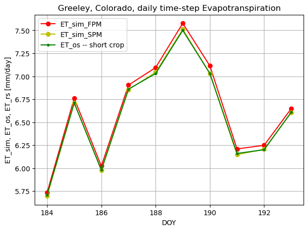
So for 24-hour time step we verified that our FPM and SPM results for short crop are matching reference data

it is noted in the reference:

ASCE-FPM, “when computed using a daily calculation timestep, was the measure against which the other equations were compared. The ASCE-FPM method, using resistance parameters as defined in Manual 70 to be functions of vegetation height and computed with a daily timestep, was the method found to perform best against lysimeter measurements in Manual 70.”

# Let's plot the data we received from methods
fig, ax1 = plt.subplots(figsize=(7,5))
# ax2 = ax1.twinx()
# ax1.plot(doy, rat_rad, 'g.-', label='Ratheor-integral')
ax1.plot(doy, ET_ref_sim_d, 'ro-', label='ET_sim_FPM')
ax1.plot(doy, ET_sim_st_d, 'yo-', label='ET_sim_SPM')
# ax1.plot(doy, radtheorint_arr, 'y', label='Rso')
if height_veg < 0.5:
    ax1.plot(doy, ET_os_daily, 'g.-', label='ET_os -- short crop')
else:
    ax1.plot(doy, ET_rs_daily, 'b.-', label='ET_rs -- tall crop')

ax1.set_ylabel('ET_sim, ET_os, ET_rs [mm/day]')
# ax2.set_ylabel('extraterrestrial radiation (Ra), [W/m^2]')
ax1.set_xlabel('DOY')
plt.title("Greeley, Colorado, daily time-step Evapotranspiration")
plt.legend(loc="upper left")
# plt.axis([0,365,0,10])
plt.grid(True)
plt.show()

In order to check that the tall crop results also match well with reference, please, consider to re-run the code above with height_veg = 0.5

1-hour timestep

We will use tall-crop in order to verify 1-hour timestep again, you can always switch to short-crop to check if it still matches the reference fine Station data for 1-hour is still the same

# Single method test based on ASCE-EWRI Appendix C, hourly time-step
# height_veg = 0.12 #vegetation height, short crop
# values for stomatal resistance rl was precalculated based on the info about resistnaces and
# nominator/denominator coefficients of the SPM
height_veg = 0.5 #tall crop
if height_veg>0.12:
    crop="tall"
    rl = 72.0 # short
else:
    crop = "short"
    rl = 66.9 #tall crop

Weather data, 1-hour timestep:

# Data from weather station
ws_Th = [30.9, 31.2, 29.1, 28.3, 26.0, 22.9, 20.1, 19.9, 18.4, 16.5, 15.4, 15.5, 13.5, 13.2, 16.2, 20.0, 22.9, 26.4, 28.2, 29.8, 30.9, 31.8, 32.5, 32.9, 32.4, 30.2, 30.6, 28.3, 25.9, 23.9]

# ws_Th_m20 = [30.9, 31.2, 29.1, 28.3, 26.0, 22.9, 20.1, 19.9, 18.4, 16.5, 15.4, 15.5, 13.5, 13.2, 16.2, 20.0, 22.9, 26.4, 28.2, 29.8, 30.9, 31.8, 32.5, 32.9, 32.4, 30.2, 30.6, 28.3, 25.9, 23.9]*0.2
ws_eah = [1.09, 1.15, 1.21, 1.21, 1.13, 1.20, 1.35, 1.35, 1.32, 1.26, 1.34, 1.31, 1.26, 1.24, 1.31, 1.36, 1.39, 1.25, 1.17, 1.03, 1.02, 0.98, 0.87, 0.86, 0.93, 1.14, 1.27, 1.27, 1.17, 1.20]
ws_Rsh = [2.24, 1.65, 0.34, 0.32, 0.08, 0.0, 0.0, 0.0, 0.0, 0.0, 0.0, 0.0, 0.0, 0.03, 0.46, 1.09, 1.74, 2.34, 2.84, 3.25, 3.21, 3.34, 2.96, 2.25, 1.35, 0.88, 0.79, 0.27, 0.03, 0.0]
ws_windspeedh = [4.07, 3.58, 1.15, 3.04, 2.21, 1.04, 0.58, 0.95, 0.30, 0.50, 1.00, 0.68, 0.69, 0.29, 1.24, 1.28, 0.88, 0.72, 1.52, 1.97, 2.07, 2.76, 2.90, 3.10, 2.77, 3.41, 2.78, 2.95, 3.27, 2.86]

ws_rhh = []
for i in range(len(ws_Th)):
    ws_svp_tmean = 0.6108 * math.exp(17.27 * ws_Th[i] / (ws_Th[i] + 237.3))
    ws_rhh.append(ws_eah[i]*100/ws_svp_tmean)

# print(ws_rhh)

# ET_os_h = [0.61, 0.48, 0.14, 0.22, 0.12, 0.04, 0.01, 0.02, 0.01, 0.01, 0.01, 0.01, 0.01, 0.01, 0.10, 0.19, 0.32, 0.46, 0.60, 0.72, 0.73, 0.79, 0.74, 0.62, 0.44, 0.35, 0.29, 0.17, 0.10, 0.07]
# ET_rs_h = [0.82, 0.66, 0.19, 0.35, 0.21, 0.06, 0.02, 0.04, 0.01, 0.01, 0.02, 0.01, 0.01, 0.01, 0.12, 0.23, 0.37, 0.52, 0.70, 0.85, 0.88, 0.97, 0.93, 0.81, 0.60, 0.52, 0.42, 0.29, 0.14, 0.10]
ET_os_h = [0.61, 0.48, 0.14, 0.22, 0.12, 0.04, 0.01, 0.02, 0.01, 0.01, 0.01, 0.01, 0.01, 0.01, 0.10, 0.19, 0.32, 0.46, 0.60, 0.72, 0.73, 0.79, 0.74, 0.62, 0.44, 0.35, 0.29, 0.17, 0.10]
ET_rs_h = [0.82, 0.66, 0.19, 0.35, 0.21, 0.06, 0.02, 0.04, 0.01, 0.01, 0.02, 0.01, 0.01, 0.01, 0.12, 0.23, 0.37, 0.52, 0.70, 0.85, 0.88, 0.97, 0.93, 0.81, 0.60, 0.52, 0.42, 0.29, 0.14]

# This data can be used toverify Radiation Calculator
SW_orig_h = [2.54, 1.96, 1.31, 0.63,  0.07, 0.0, 0.0, 0.0, 0.0, 0.0, 0.0, 0.0, 0.0, 0.04, 0.56, 1.24, 1.90, 2.49, 2.97, 3.32, 3.50, 3.51, 3.34, 3.01, 2.54, 1.96, 1.31, 0.63, 0.07]
Ra_orig_h = [3.26, 2.52, 1.68, 0.81, 0.09, 0.0, 0.0, 0.0, 0.0, 0.0, 0.0, 0.0, 0.0, 0.05, 0.72, 1.59, 2.43, 3.19, 3.81, 4.26, 4.49, 4.51, 4.29, 3.87, 3.26, 2.52, 1.68, 0.81, 0.09]
LW_orig_h =[0.284, 0.262, 0.017, 0.017, 0.017, 0.016, 0.015, 0.015, 0.015, 0.014, 0.014, 0.014, 0.014, 0.014, 0.014, 0.223, 0.244, 0.278, 0.299, 0.331, 0.308, 0.0332, 0.315, 0.248, 0.134, 0.084, 0.147, 0.143, 0.143]
Rnet_orig_h = [1.441, 1.009, 0.244, 0.229, 0.044, -0.016, -0.015, -0.015, -0.015, -0.014, -0.014, -0.014, -0.014, 0.009, 0.340, 0.616, 1.096, 1.524, 1.888, 2.171, 2.164, 2.239, 1.964, 1.485, 0.905, 0.593, 0.461, 0.065, -0.12]

We create timeseries from weather data:

# reference data is 30-hours from 1-07-2000 16.00 to 2-07-2000 21.00
nhour = 30 # nr of time steps
t_starth = utc.time(2000, 7, 1,16,0,0,0) # starting point, 1-07-2000 16.00
dthours = deltahours(1) # returns daily timestep in seconds


# Let's now create Shyft time series from the supplied lists of precipitation and temperature.
# First, we need a time axis, which is defined by a starting time, a time step and the number of time steps.
tah = TimeAxis(t_starth, dthours, nhour) # days
# print(len(tah))


# First, we convert the lists to shyft internal vectors of double values:
temph_dv = DoubleVector.from_numpy(ws_Th)
eah_dv = DoubleVector.from_numpy(ws_eah)
rsh_dv = DoubleVector.from_numpy(ws_Rsh)
windspeedh_dv = DoubleVector.from_numpy(ws_windspeedh)

rhh_dv = DoubleVector.from_numpy(ws_rhh)

# Finally, we create shyft time-series as follows:
# (Note: This step is not necessarily required to run the single methods.
#  We could also just work with the double vector objects and the time axis)
temph_ts = TimeSeries(tah, temph_dv, point_fx=instant)
eah_ts = TimeSeries(tah, eah_dv, point_fx=instant)
rsh_ts = TimeSeries(tah, rsh_dv, point_fx=instant)
windspeedh_ts = TimeSeries(tah, windspeedh_dv, point_fx=instant)


#recalculated inputs:
rhh_ts = TimeSeries(tah, rhh_dv, point_fx=instant)

Create Radiation Caclulator, you can skip this step, if your intention is to verify evapotranspiration only:

land_albedo = 0.26
turbidity = 1.0
radph = api.RadiationParameter(land_albedo,turbidity)
radch = api.RadiationCalculator(radph)
radrh =api.RadiationResponse()

Create FPM and SPM Calculators:

method_option = True # FPM
# pmph=api.PenmanMonteithParameter(lai,height_ws,height_t)
pmph=api.PenmanMonteithParameter(height_veg,height_ws,height_t, rl,method_option)
pmch=api.PenmanMonteithCalculator(pmph)
pmrh =api.PenmanMonteithResponse()

method_option = False # SPM
pmphst=api.PenmanMonteithParameter(height_veg,height_ws,height_t, rl,method_option)
pmchst=api.PenmanMonteithCalculator(pmphst)
pmrhst =api.PenmanMonteithResponse()

We will also compare the FPm and SPM methods to the Priestley-Taylor (PT) implementation So, need to create PT calculator

#PriestleyTaylor
ptp = api.PriestleyTaylorParameter(0.2,1.26)
ptc = api.PriestleyTaylorCalculator(0.2, 1.26)
ptr = api.PriestleyTaylorResponse

Let’s run the simulation:

ET_ref_sim_h= []
ET_sim_st_h = []

timeofday = []
ET_pt_sim_h = []
Rso_sim_h = []
LW_sim_h = []
SW_sim_h = []
Ra_sim_h = []
Rnet_sim_h = []

for i in range(nhour-1):
    timeofday.append(datetime.fromtimestamp(tah.time_points[i]))
    # Radiation methods
    radch.net_radiation_step_asce_st(radrh, latitude, tah.time(i), deltahours(1),slope_deg, aspect_deg, temph_ts.v[i], rhh_ts.v[i], elevation, rsh_ts.v[i]/c_MJm2h2Wm2 )
    # collect radiation results
    Ra_sim_h.append(radrh.ra*c_MJm2h2Wm2*24 )
    Rso_sim_h.append(radrh.sw_t * c_MJm2h2Wm2)
    SW_sim_h.append(radrh.sw_t*c_MJm2h2Wm2)
    LW_sim_h.append(radrh.net_lw*c_MJm2h2Wm2)
    Rnet_sim_h.append(radrh.net * c_MJm2h2Wm2)
    # Penman-Monteith methods
    # SPM
    pmchst.reference_evapotranspiration(pmrhst,deltahours(1),Rnet_orig_h[i],temph_ts.v[i],temph_ts.v[i],rhh_ts.v[i],elevation,windspeedh_ts.v[i])
    # FPM
    pmch.reference_evapotranspiration(pmrh, deltahours(1),Rnet_orig_h[i], temph_ts.v[i],temph_ts.v[i],  rhh_ts.v[i], elevation,windspeedh_ts.v[i])
    # Collect results
    ET_ref_sim_h.append(pmrh.et_ref)
    ET_sim_st_h.append(pmrhst.et_ref)
    # ET_pt_sim_h.append(ptc.potential_evapotranspiration(temph_ts.v[i], radrh.rnet, rhh_ts.v[i]*0.01)*3600) # the PT calculates [mm/s]
    ET_pt_sim_h.append(ptc.potential_evapotranspiration(temph_ts.v[i], ws_Rsh[i]/c_MJm2h2Wm2,rhh_ts.v[i] * 0.01) * 3600)  # the PT calculates [mm/s]

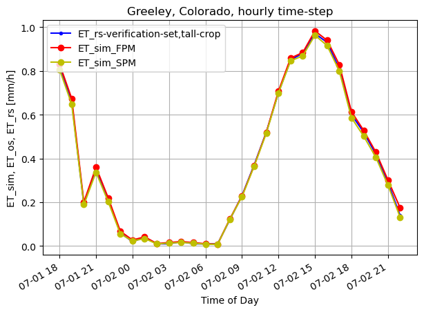
We will now plot some results. We did simulation for tall-crop.

summary = 0
for i in range(len(ET_ref_sim_h)):
    summary+=math.fabs(ET_ref_sim_h[i]-ET_sim_st_h[i])

mae = (math.sqrt(summary/len(ET_ref_sim_h)))
print('MAE:' + str(mae))

fig, ax1 = plt.subplots(figsize=(7,5))
# ax2 = ax1.twinx()
# ax1.plot(doy, rat_rad, 'g.-', label='Ratheor-integral')
if height_veg>0.12:
    ax1.plot(timeofday, ET_rs_h, 'b.-', label='ET_rs-verification-set,'+crop+'-crop') #tall
else:
    ax1.plot(timeofday, ET_os_h, 'b.-', label='ET_os-verification-set,'+crop+' crop') #short

ax1.plot(timeofday, ET_ref_sim_h, 'ro-', label='ET_sim_FPM')
ax1.plot(timeofday, ET_sim_st_h, 'yo-', label='ET_sim_SPM')
# ax1.plot(doy, radtheorint_arr, 'y', label='Rso')


# ax1.plot(timeofday, ET_pt_sim_h, 'k.-', label='ET_sim_pt')

ax1.set_ylabel('ET_sim, ET_os, ET_rs [mm/h]')
# ax2.set_ylabel('extraterrestrial radiation (Ra), [W/m^2]')
ax1.set_xlabel('Time of Day')
plt.title("Greeley, Colorado, hourly time-step")
plt.legend(loc="upper left")
# plt.axis([0,365,0,10])
plt.gcf().autofmt_xdate()
plt.grid(True)
plt.show()

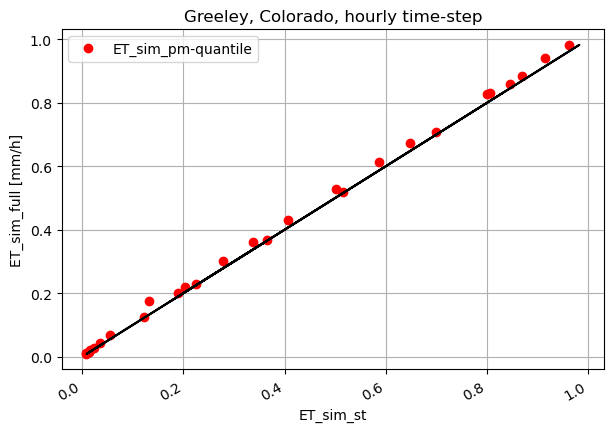
fig, ax1 = plt.subplots(figsize=(7,5))
ax1.plot(ET_sim_st_h, ET_ref_sim_h, 'ro', label='ET_sim_pm-quantile')
ax1.plot(ET_ref_sim_h, ET_ref_sim_h, 'k')

ax1.set_ylabel('ET_sim_full [mm/h]')
# ax2.set_ylabel('extraterrestrial radiation (Ra), [W/m^2]')
ax1.set_xlabel('ET_sim_st')
plt.title("Greeley, Colorado, hourly time-step")
plt.legend(loc="upper left")
# plt.axis([0,365,0,10])
plt.gcf().autofmt_xdate()
plt.grid(True)
plt.show()

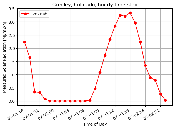
The following peace is to see the radiation results:

We are very close to the ASCE-EWRI project, though Radiation model is take from newer document:

ref.: Allen, Richard G.; Trezza, Ricardo; Tasumi, Masahiro;

Analytical integrated functions for daily solar radiation on slopes, Agricultural and Forest Meteorology,2006

fig, ax1 = plt.subplots(figsize=(7,5))
ax1.plot(timeofday, ws_Rsh[0:29], 'ro-', label='WS Rsh')
# ax1.plot(timeofday, Rnet_orig_h, 'g.-', label='Rnet_orig')
ax1.set_ylabel('Measured Solar Radiation [MJ/m2/h]')
ax1.set_xlabel('Time of Day')
plt.title("Greeley, Colorado, hourly time-step")
plt.legend(loc="upper left")
# plt.axis([0,365,0,10])
plt.gcf().autofmt_xdate()
plt.grid(True)
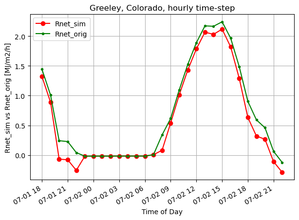
fig, ax1 = plt.subplots(figsize=(7,5))
ax1.plot(timeofday, Rnet_sim_h, 'ro-', label='Rnet_sim')
ax1.plot(timeofday, Rnet_orig_h, 'g.-', label='Rnet_orig')
ax1.set_ylabel('Rnet_sim vs Rnet_orig [MJ/m2/h]')
ax1.set_xlabel('Time of Day')
plt.title("Greeley, Colorado, hourly time-step")
plt.legend(loc="upper left")
# plt.axis([0,365,0,10])
plt.gcf().autofmt_xdate()
plt.grid(True)
# # #
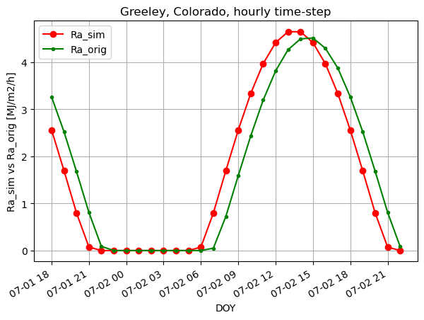
fig, ax1 = plt.subplots(figsize=(7,5))
ax1.plot(timeofday, Ra_sim_h, 'ro-', label='Ra_sim')
ax1.plot(timeofday, Ra_orig_h, 'g.-', label='Ra_orig')
ax1.set_ylabel('Ra_sim vs Ra_orig [MJ/m2/h]')
ax1.set_xlabel('DOY')
plt.title("Greeley, Colorado, hourly time-step")
plt.legend(loc="upper left")
# plt.axis([0,365,0,10])
plt.gcf().autofmt_xdate()
plt.grid(True)
# #
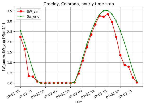
fig, ax1 = plt.subplots(figsize=(7,5))
# ax2 = ax1.twinx()
ax1.plot(timeofday, SW_sim_h, 'ro-', label='SW_sim')
# ax1.plot(doy, radtheorint_arr, 'y', label='Rso')
ax1.plot(timeofday, SW_orig_h, 'g.-', label='Sw_orig')
ax1.set_ylabel('SW_sim vs SW_orig [MJ/m2/h]')
ax1.set_xlabel('DOY')
plt.title("Greeley, Colorado, hourly time-step")
plt.legend(loc="upper left")
# plt.axis([0,365,0,10])
plt.gcf().autofmt_xdate()
plt.grid(True)
#
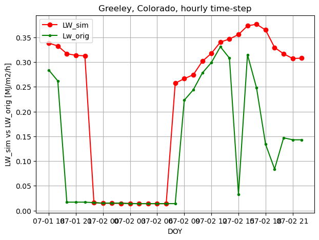
fig, ax1 = plt.subplots(figsize=(7,5))
# ax2 = ax1.twinx()
ax1.plot(timeofday, LW_sim_h, 'ro-', label='LW_sim')
# ax1.plot(doy, radtheorint_arr, 'y', label='Rso')
ax1.plot(timeofday, LW_orig_h, 'g.-', label='Lw_orig')
ax1.set_ylabel('LW_sim vs LW_orig [MJ/m2/h]')
ax1.set_xlabel('DOY')
plt.title("Greeley, Colorado, hourly time-step")
plt.legend(loc="upper left")
# plt.axis([0,365,0,10])
plt.grid(True)