Constructing a model using the Shyft API
Setup environment for tutorials
Introduction
Aim of this tutorial is to introduce a Shyft user to Shyft’s API. The Shyft API provides all functionality needed to construct a model, calibrate it, and run it. It is also a great way of learing about the “Shyftonic” way of thinking, i.e. getting to know the architecture of Shyft.
In order to get to know the Shyft API, a very simple model will be constructed in the course of this tutorial. The model will be fed with test data, run, and calibrated. In the end it is shown how data can be extracted from the model.
To define a model domain, Shyft uses a number of geo-located sub-units, the cells. Each cell has certain properties like land type fractions (glacier fraction, forest fraction, etc.), area, and geo-location. Cells that belong to the same (sub)catchment have the same catchment ID. The simple model we will construct herein will only hold 1 cell, in order to keep the programming effort at a minimum. Nevertheless will the tutorial provide you with the skills needed to setup more complex model domains, existing of several catchments, each composed from a large number of cells.
STEP 0.1: LOAD AND PLOT TEST DATA
Prior to digging into the Shyft API, we will initialize the test dataset. By initiating the TestData Class, a dataset providing all input variables needed to run a hydrological simulation is constructed.
The variables needed to run a model provided by Shyft are standard meteorologic variables: temperature, precipitation, wind speed, relative humidity, and radiation.
In addition to those variables, observed discharged and the total catchment area are provided by the dataset. For now, these information will be enough to construct a simple model aiming to simulate the discharge of the region.
Start by importing test data, modify test_data_path if needed.
import numpy as np
import pandas as pd

from shyft import time_series as api

test_data_path = "/workspaces/shyft-doc/sphinx/notebooks/shyft-intro-course-master/test_data/"

class TestData():
    def __init__(self):
        self.met_filename = test_data_path + "06191500_lump_cida_forcing_leap.txt"
        self.streamflow_filename = test_data_path + "06191500_streamflow_qc.txt"
        self._station_info, self._df_met = self._get_met_data_from_camels_database()
        self._df_streamflow = self._get_streamflow_data_from_camels_database()
        self.temperature = self._df_met['temperature'].values
        self.precipitation = self._df_met['precipitation'].values
        self.radiation = self._df_met['radiation'].values
        self.relative_humidity = self._df_met['relative_humidity'].values
        self.wind_speed = self._df_met['wind_speed'].values
        self.time = self._df_met['time'].values
        self.discharge = self._df_streamflow.discharge
        self.area = self._station_info['area']
        # TODO assure time is same; assure same length of all;


    def _get_met_data_from_camels_database(self):
        station_info = {}
        with open(self.met_filename) as data:
            station_info['lat'] = float(data.readline())  # latitude of gauge
            station_info['z'] = float(data.readline())  # elevation of gauge (m)
            station_info['area'] = float(data.readline())  # area of basin (m^2)
        keys = ['Date', 'dayl', 'precipitation', 'radiation', 'swe', 'tmax', 'tmin', 'vp']
        df = pd.read_table(self.met_filename, skiprows=4, names=keys)
        df["temperature"] = (df["tmin"] + df["tmax"]) / 2.
        df.pop("tmin")
        df.pop("tmax")
        df["precipitation"] = df["precipitation"] / 24.0 # mm/h
        df["wind_speed"] = df["temperature"] * 0.0 + 2.0  # no wind speed in camels
        df["relative_humidity"] = df["temperature"] * 0.0 + 0.7  # no relative humidity in camels
        df["time"] = self._get_utc_time_from_daily_camels_met(df['Date'].values)
        return station_info, df

    def _get_streamflow_data_from_camels_database(self):
        keys = ['sgid','Year','Month', 'Day', 'discharge', 'quality']
        df = pd.read_table(self.streamflow_filename, names=keys, delim_whitespace=True)
        time = self._get_utc_time_from_daily_camels_streamgauge(df.Year, df.Month, df.Day)
        df['time'] = time
        df.discharge.values[df.discharge.values == -999] = np.nan
        df.discharge = df.discharge * 0.0283168466  # feet3/s to m3/s
        #df.discharge[df.discharge == -999] = np.nan  # set missing values to nan
        return df

    def _get_utc_time_from_daily_camels_met(self, datestr_lst):
        utc = api.Calendar()
        time = [utc.time(*[int(i) for i in date.split(' ')]).seconds for date in datestr_lst]
        return np.array(time) - 12*3600 # shift by 12 hours TODO: working nicer?

    def _get_utc_time_from_daily_camels_streamgauge(self, year, month, day):
        utc = api.Calendar()
        time = [utc.time(int(y), int(m), int(d)).seconds for y,m,d in zip(year, month, day)]
        return np.array(time)

data = TestData() # constructs an instance of the TestData Class...
STEP 0.2 - Inspect data
Continue with importing the Shyft API. The Shyft API gives access to all functionality needed to construct a model. We can import it via …
import shyft.hydrology as api # import the Shyft hydrlogy  API
import shyft.time_series as sts # import Shyft time series
In addition to the Shyft API, we will import some modules that ease the handling of arrays (numpy module) and plotting (matplotlib library). Besides this, we also import a ready-to-use dataset that provides us with test data that we will use to run the hydrological model.
import numpy as np # for handling arrays
from matplotlib import pyplot as plt # for plotting
We are now set up to use the API for constructing a model. But first let’s take a quick look to the test data we will be using to drive the model.
fig, ax = plt.subplots(3, figsize=(15,10))
ax[0].plot(data.temperature, label='temperature [deg C]')
ax[0].legend(loc=1)
ax[1].plot(data.precipitation, label='precipitation [mm/h]')
ax[1].legend(loc=1)
ax[2].plot(data.radiation, label='radiation [W/2]')
ax[2].legend(loc=1)
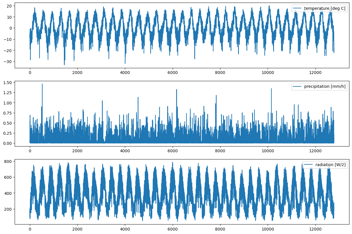
We have plotted the test data without time reference. The corresponding time vector is also provided by TestData.
print(data.time)
# The time is given as UTC timestamp (seconds since January 1 1970). In this exmaple, the delta t between
# time points is 60*60*3600 seconds. Thus, the dataset provides daily values. By convention, the first data value
# gives the average value defined by the time span between the first and the second time points given in the time vector.

# output: [ 315532800  315619200  315705600 ... 1419811200 1419897600 1419984000]
STEP 1: CHOOSE A MODEL
Shyft has different model types to offer, each of which is composed of a unique sequence of hydrological methods. We will use the pt_gs_k model, consisting of the Priestly Taylor equation to calculate potential evaportanspiration (PT), a gamma-function based snow routine (GS), and the Kircher method to calculate the discharge response (K).
model_type = api.pt_gs_k.PTGSKModel

# Further model options are:

#model_type = api.pt_ss_k.PTSSKModel
#model_type = api.pt_ss_k.PTHSKModel
#model_type = api.hbv_stack.HbvOptModel
#model_type = api.pt_gs_k.PTGSKOptModel
STEP 2: DEFINE THE MODEL DOMAIN
Region, catchment, and cells in Shyft: Configuring the model domain
A Shyft model domain is constructed from cells, which are grouped to catchments using a catchment ID. A cell is characterized by a mid-point (x,y,z), area, land type fractions (glacier, forest, etc), and assigned to a catchment via a catchment ID.
Let’s construct a cell:
x, y, z = 0, 0, 0  # cell center coordinates [m]
area = data.area  # cell area [m2]
cid = 1  # cell's catchment ID
mid_point = api.GeoPoint(x, y, z) # mid point
glacier = 0.0  # areal glacier fraction
lake = 0.0
reservoir = 0.0
forest = 0.0
unspecified = 1.0  # residual: 1 - glacier - lake - reservoir - forest
radiation_slope_factor = 1.0  # A factor to correct radiation input according to the cells orientation
ltf = api.LandTypeFractions(glacier, lake, reservoir, forest, unspecified)  # Class to handle land type fractions
geo_cell_data = api.GeoCellData(mid_point, area, cid, radiation_slope_factor, ltf)  # Handls all cell data
cell = model_type.cell_t()  # Constructing a cell
cell.geo = geo_cell_data  # Feeding the cell with data

# Append cells to a cell vector... here only shown for the one cell. In more complex scenarios, many more cells are used to define a domain.
cell_vector = model_type.cell_t.vector_t()
cell_vector.append(cell)
STEP 3: CONFIGURE THE MODEL
Model specific parameters define how the model equations will respond to a certain meteorological forcing. As the parameters are specific to the model type, we can get the correct parameters directly from the model class.
We differ between region parameters (all cells in a domain have the same parameters), and catchment parameters (certain (sub)catchments of the domain can be characterized by a set of model parameters different than the region parameters).
Let’s construct region parameters suiting our model.
region_parameter = model_type.parameter_t() # constructing region parameters

# and also catchment parameters
catchment_parameters = model_type.parameter_t.map_t() # Constructing a parameter map, that maps a set of parameters to a catchment ID
catchment_parameters[1] = region_parameter # same type as region parameters. We map catchment parameters to the cell with catchment ID 1
STEP 4: CONSTRUCT THE REGION MODEL
The region model combines information about the model domain, or region, which is provided by the cells, and the model we want to use. The link between a region and the model are the region (or catchment) specific model parameters.
region_model = model_type(cell_vector, region_parameter, catchment_parameters) # needs all the information from above
STEP 5: FEED FORCING DATA TO THE REGION MODEL BY CONSTRUCTING A REGION ENVIRONMENT
Before running a simulation, we need to feed forcing data to the region model. This is done by constructing forcing data time series that are geo-located, so called “sources”. In order to create time series of forcing data, we need to define a time axis, and then combine it with the data values.
In order to add sources to the region model, collections of sources of a certain type (temperature, precipitation, …) are organized in SourceVectors. These SourceVectors are then added to the region model.
We first initiate a time-axis from the time points to which the source data corresponds by first constructing a time vector, …
time_vec = sts.UtcTimeVector(data.time) # convert the interger array to a shyft time vector
… and then constructing a time axis:
A time axis if a set if non-overlapping periods. The time points give the start and end points of those periods. In order to have the same amount of perdios as data values, we need to add one more time point in order to mark the end point of the last period of the time axis. Since the time resolution of our data is daily, we simply add 60*60*24 seconds to the last time point provided to define the end point of the last interval.
time_end = time_vec[-1] + 60*60*24 # end of last time interval
We now have all information needed to construct a time axis …
ta_srs = sts.TimeAxisByPoints(time_vec, t_end=time_end)
… and make a time series by combining the data values with the corresponding time axis.
Since the data values represent daily average values, we tell the constructor that it should interprete the values as avarage values, by using the point interpretation policy provided by Shyft’s API (api.POINT_AVERAGE_VALUE). Another option would be api.POINT_INSTANT_VALUE, used in cases where the measured values represent instant values
t_ts = sts.TimeSeries(ta_srs, api.DoubleVector.from_numpy(data.temperature), sts.POINT_AVERAGE_VALUE) # time series
We then do exactly the same for rest of the model forcing variables:
p_ts = sts.TimeSeries(ta_srs, api.DoubleVector.from_numpy(data.precipitation), sts.POINT_AVERAGE_VALUE)
ws_ts = sts.TimeSeries(ta_srs, api.DoubleVector.from_numpy(data.wind_speed), sts.POINT_AVERAGE_VALUE)
rh_ts = sts.TimeSeries(ta_srs, api.DoubleVector.from_numpy(data.relative_humidity), sts.POINT_AVERAGE_VALUE)
r_ts = sts.TimeSeries(ta_srs, api.DoubleVector.from_numpy(data.radiation), sts.POINT_AVERAGE_VALUE)
We now declare the geo locations of our time series. For simplicity, we just use the same location for all time series. The coordinates must to be based on an orthogonal corrdinate system (e.g. UTM).
geop = api.GeoPoint(0,0,0) # x,y,z location
Finally, we have all information needed to construct variable-type specific sources by linking geo location and time series:
t_srs = api.TemperatureSource(geop, t_ts)
p_srs = api.PrecipitationSource(geop, p_ts)
ws_srs = api.WindSpeedSource(geop, ws_ts)
rh_srs = api.RelHumSource(geop, rh_ts)
r_srs = api.RadiationSource(geop, r_ts)
In this example, we just provide one source per input variable.
However, the most common case is that we have many geo-located time series per forcing variable, e.g. from several obervational stations in a region or from a gridded forcing data set (numerical weather forecasting model, climate model, gridded observations, etc).
Before we can feed the sources to the model, we therefore need to construct source vectors, which are collections of sources of the same variable type (temperature, precipitation, …).
Again: for simplicity only one source per vector is appended in this example. Accordingly, many sources with different geo locations could be added to the same vector.
# constructing the source vectors
t_srs_vec = api.TemperatureSourceVector([t_srs])
p_srs_vec = api.PrecipitationSourceVector([p_srs])
ws_srs_vec = api.WindSpeedSourceVector([ws_srs])
rh_srs_vec = api.RelHumSourceVector([rh_srs])
r_srs_vec = api.RadiationSourceVector([r_srs])
All information about sources is organized in the region environment. The region environment is the part of the region model and contains all geo-located sources.
# constructing a region environment from the environment sources:
region_env = api.ARegionEnvironment()
region_env.temperature = t_srs_vec
region_env.precipitation = p_srs_vec
region_env.wind_speed = ws_srs_vec
region_env.rel_hum = rh_srs_vec
region_env.radiation = r_srs_vec
Now that we have created a region environment holding all geo-located time series that we want to use as model forcing, we are ready to update the region model with the freshly costructed region environment:
region_model.region_env = region_env
STEP 6: RUNNING THE MODEL
In order to be able to run the model, two more requirements need to be fulfilled:
1. Initial values for state variables need to be defined. The starting state needs to be defined in order to make future predictions of the model state, e.g., tomorrow’s amount of snow in a cell can only be calculated if today’s amount of snow is known. The amount of snow is a typical state variable and needs to be set prior to a model run in order to enable a quality calculation forward in time.
2. Since the model-stack is executed cell-by-cell, the source variables (or model forcing variables: temperature, etc..) need to be interpolated from the source locations to the cell locations, so that each cell holds a complete set of forcing variables. These are then used to run the model cell-by-cell.
After providing these steps, the model is ready to run.
1. The starting model state: updating the current state of the model
We first construct a state that suits to the model. The state will be constructed with default values for each state varibale.
state = region_model.state_t()
We can update state variables by simply setting the variables to desired values.
state.kirchner.q = 0.8 # Setting the initial discharge value of the kirchner routine
The model needs to keep track of which state belongs to which cell. This can be achieved using the state_with_id state type. You can think of it as a geo-referenced model state, mapping a certain state to a cell. A collection of states_with_id can be managed with a state_with_id_vct, the state_with_id vector.
state_with_id = region_model.state_with_id_t() # constructing the state_with_id
state_with_id_vct = region_model.state_with_id_t.vector_t() # constructing the state_with_id vector
state_with_id.state = state # set the state
state_with_id.id = state_with_id.cell_state(cell.geo) # mapping it to the cell
state_with_id_vct.append(state_with_id) # append it to the vector. As we only constructed a one-cell model at the moment,
                                        # we only need to append this one cell.
We now can update the region model with the cell states, by passing the state vector to the apply_state() method. Only cells that have a catchment ID that is member of the list passed as second argument are updated.
region_model.state.apply_state(state_with_id_vct, [1])
Let’s check if the value of the state variable that we just tried to update is actually applied.
print(region_model.current_state[0].kirchner.q)
# output: 0.8
The current state will change as the model steps forward in time and always represent the model state after the last time stepping. Because it changes, it makes sense to store the initial state (which is to this point the current state of the model), so that it later can be re-set as current state, e.g. in order to repeat simulations under the same conditions.
region_model.initial_state = region_model.current_state
Since computation time is costly, it is possible to disable/enable the collection of state variables for catchments. Disabling state collection leads to a faster performance of the model, however, the time series of state variables are not stored in memmory during a model run, and thus not accessible after a simulation. Let’s enable state collection for this simulation.
region_model.set_state_collection(1, True) # Enabling state collection for all cells with catchment ID 1
2. Running the interpolation
Before running the interpolation, we need to initiate the cell environment. This constructs the environment variables at the cell level at the temporal resolution of a time axis argument.
After initiation, all values of the environment variables at the cell level are set to zero.
The interpolation step will then fill each cell’s environment variable time series based on the time series provided in the sources, and in dependence of a set of interpolation parameters, that define how the interpolation is conducted.
Let’s first construct the simulation time axis …
utc = sts.Calendar() # shyft.api calendar, nice for keeping track of time
n_steps = 365*20 # number of steps
ta_sim = sts.TimeAxis(utc.time(1990, 9, 1, 0, 0, 0), sts.deltahours(24), 365*20)  # simulation time axis, 20 year at daily resolution
… and then initialize the cell environment:
region_model.initialize_cell_environment(ta_sim)
Let’s now run the interpolation:
The interpolation spatially and temporally interpolates the environment variables from sources (charcterized by the by time axis ta_srs and geo-location) to the cells (characterized by time axis ta_sim and the cell’s mid-point). The region_model was constructed with default interpolation parameters, which we can use for the interpolation.
region_model.interpolate(region_model.interpolation_parameter, region_model.region_env)
# output: True
3. Running the model
Let’s finally run the model forward in time, as defined by time axis ta_sim.
region_model.run_cells()
STEP 7: EXTRACTING SIMULATION RESULTS
Model results (and states) are stored in memmory (and not written to file, as you might know it from other models) and can be accessed via the region model. Results can be accessed cell-by-cell, or aggregated at the catchment level. The latter is calculated on demand. A list of catchment IDs can be passed that define which cells should be included in the aggregation.
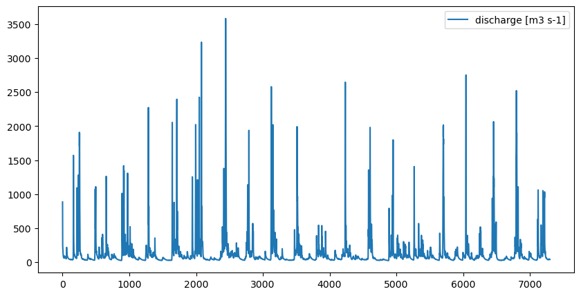
Some of the results can be accessed via the “statistics” attribute of the region model. Let’s have a look at the discharge:
q = region_model.statistics.discharge([1]) # A TimeSeries object is returned: the discharge aggregated over cells with ID 1
                                           # Reminder: We have already learned about TimeSeries further up
The values of a TimeSeries object can be accessed as follows:
q_vals = q.values
# Let's plot the discharge
fig, ax = plt.subplots(figsize=(10,5))
ax.plot(q_vals, label="discharge [m3 s-1]")
ax.legend()
So far, the model has been run with default model parameters. Let’s now calibrate the model.
STEP 8: MODEL CALIBRATION
In order to estimate model parameters, a discharge time series is required that is used to evaluate the simulated discharge.
The test dataset offers observed discharge for the test region. Let’s use it to create the evaluation time series, the so called target:
# Target time series from all discharge observations available:
ts_trg_all = sts.TimeSeries(ta_srs, data.discharge, sts.POINT_AVERAGE_VALUE)
If we would like to limit the evaluation to only a part of the simulation, we can subset the target time series by defining a new time axis, that only covers a part of the simulation period:
# subset time series to desired time axis for calibration
ta_trg = sts.TimeAxis(utc.time(1991, 9, 1, 0, 0, 0), sts.deltahours(24), 365*18)  # simulation time axis, 18 years
ts_trg = ts_trg_all.average(ta_trg)
The model needs to know the area that is represented by the target time series. For this reason, “target specifications” are used to combine a target time series with additional properties characterizing the target:
# make target specification vector
calc_type = api.TargetSpecCalcType(0) # Which goal function you want to use; 0 is Nash-Sutcliffe
cids = api.IntVector.from_numpy([1]) # a list with IDs to let the model know which catchments the target represents
weight = 1 # Here we have only one target time series. If you have many, you need to tell the model how to weighten them during calibration
target_specification = api.TargetSpecificationPts(ts_trg, cids, weight, calc_type) # construct the target specification
You can make as many target specifications as you want. They can represent different areas and cover different periods. A collection of target specifications is organized via target specification vectors:
target_spec_vec = api.TargetSpecificationVector()
target_spec_vec.append(target_specification)
As the model will run simulations over and over again during calibration in order to try out differnt parameter sets, it is advantageous if the model runs as fast as possible. Collecting time series of state and response variables slows a model down. As many of these variables are not needed during calibration (e.g. herein, we only use discharge to calibrate the model), Shyft offers an optimized model type that can be used for calibration. This model will discard most of the response and state variables as it steps forwards in time. You can construct an optimized model from the already ready-to-use region model:
region_model_opt = region_model.create_opt_model_clone()
In order to run a calibration, we also need to define the parameter ranges between which the optimization routine should search for an optimal parameter. Let’s construct 3 region model parameter sets: one to define the lower bound parameters, one to define the upper bound parameters, and one which gives the starting values of the parameters, from which an optimization run will start.
p_min = region_model_opt.parameter_t()
p_max = region_model_opt.parameter_t()
p_init = region_model_opt.parameter_t()
So far, the parameter objects are filled with default values. Let’s set the ranges of some key parameters…
# make a difference in parameter range
p_min.kirchner.c1, p_max.kirchner.c1, p_init.kirchner.c1 = -8, -1, -3  # kirchner response parameter
p_min.kirchner.c2, p_max.kirchner.c2, p_init.kirchner.c2 = 0.05, 1.0, 0.4  # kirchner response parameter
p_min.kirchner.c3, p_max.kirchner.c3, p_init.kirchner.c3 = -1, -0.01, -1.0  # kirchner response parameter

p_min.gs.tx, p_max.gs.tx, p_init.gs.tx = -3, 5, 0  # gamma snow, rain/snow threshold temperature [deg. C]
p_min.gs.wind_const, p_max.gs.wind_const, p_init.gs.wind_const = 0, 3, 1.5  # wind scaling for turbulent flux calculations
p_min.gs.wind_scale, p_max.gs.wind_scale, p_init.gs.wind_scale = 1, 6, 3  # wind scaling for turbulent flux calculations

p_min.p_corr.scale_factor, p_max.p_corr.scale_factor, p_init.p_corr.scale_factor = 0.5, 1.2, 1  # precipitation scaling

p_min.ae.ae_scale_factor, p_max.ae.ae_scale_factor, p_init.ae.ae_scale_factor = 0.5, 1.5, 1 # actual evapo scaling
Each optimized model offers an optimizer Class that offers functionality to run an automized calibration. Let’s construct it:
optimizer = api.pt_gs_k.PTGSKOptModel.optimizer_t(region_model_opt)
Remember the target we specified earlier? Let’s make the otimizer aware of the target, parameter ranges, and the parameter starting values:
optimizer.target_specification = target_spec_vec
optimizer.parameter_lower_bound = p_min
optimizer.parameter_upper_bound = p_max
optimizer.set_verbose_level(1)
We finally can run a calibration!
The optimizer will return an optimized set of parameters once it found the (hopefully) best set of parameters:
print("Calibrating ...")
opt_params = optimizer.optimize(p_init, 1500, 0.2, 1e-5) # calibrateing ... this can take a little while...
print("... done!")
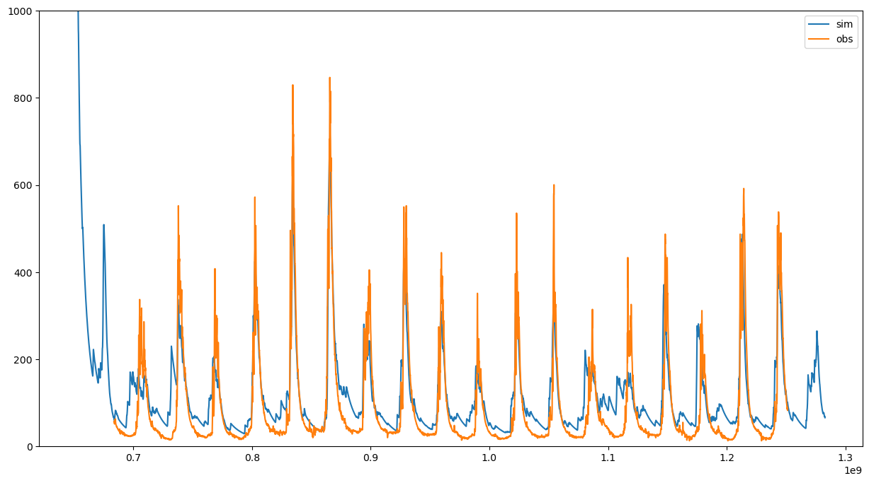
Let’s run the model one more time. This time with optimized parameters:
# Running the model with optimized parameters
NSE = 1-optimizer.calculate_goal_function(opt_params)
print("Nash-Sutcliffe efficiency: ", NSE)
# output: 0.7299080206036372
# Accessing the simulated discharge ...
q_opt = region_model_opt.statistics.discharge([])

# and plot it, together with the observed discharge:
fig, ax = plt.subplots(figsize=(15,8))
ax.plot(q_opt.time_axis.time_points[:-1], q_opt.values, label='sim')
ax.plot(ts_trg.time_axis.time_points[:-1], ts_trg.values, label='obs')
ax.set_ylim([0, 1000])
ax.legend()
You’re done! You should be able to setup your own Shyft region model, calibrate it, and access simulated data. Try it out:
Exercise
Construct a region model with 4 cells. Cell 1 and 2 should have catchment ID 1 and cell 3 and 4 should have catchment ID 2, and the following properties: * cell 1 should have an area of 3390 km2, x=0, y=0, z=0 * cell 2 should have an area of 565 km2, x=80000, y=0, z=0 * cell 3 should have an area of 2260 km2, x=0, y=80000, z=0 * cell 4 should have an area of 565 km2, x=80000, 80000, z=0
There are no glaciers, lakes, and reservoirs in the region, but cell 1 is to 50% covered by forest.
Find an optimized set of model parameters for the region (assume that he observed discharge represents the combined discharge of catchment 1 and 2).
Use the optimized region parameters from the calibration in order to simulate the discharge of the region, and of catchment 1 and 2.