Configured Shyft simulations
Setup environment for tutorials
Introduction
Shyft provides a toolbox for running hydrologic simulations. As it was designed to work in an operational environment, we’ve provided several different workflows for running a model simulation. The main concept to be aware of is that while we demonstrate and build on the use of a ‘configuration’, nearly all simulation functionality is also accessible with pure python through access to the API. This is the encouraged approach to simulation. The use of configurations is intended to be a mechanism of running repeated operational simulations when one is interested in archiving and storing (potentially to a database) the specifics of the simulation.
Below we start with a high level description using a configuration object, and in Part 2 <TutorialNidelvaPart1> of the simulation notebooks we describe the approach using the lower level APIs. It is recommended, if you intend to use Shyft for any kind of hydrologic exploration, to become familiar with the API functionality.
This notebook briefly runs through the simulation process for a pre-configured catchment. The following steps are described:
Loading required python modules and setting path to Shyft installation
Configuration of a Shyft simulation
Running a Shyft simulation
Post-processing: Fetching simulation results from the simulator-object.
1. Loading required python modules and setting path to Shyft installation
Shyft requires a number of different modules to be loaded as part of the package. Below, we describe the required steps for loading the modules, and note that some steps are only required for the use of the tutorial.
# Pure python modules and jupyter functionality
# first you should import the third-party python modules which you'll use later on
# the first line enables that figures are shown inline, directly in the notebook
%matplotlib inline
import os
import datetime as dt
import pandas as pd
from os import path
import sys
from matplotlib import pyplot as plt
The Shyft Environment
Set shyft_data_path:
# try to auto-configure the path, -will work in all cases where doc and data
# are checked out at same level
from shyft.hydrology import shyftdata_dir

shyft_data_path = os.path.abspath("/workspaces/shyft-data/")
if path.exists(shyft_data_path) and 'SHYFT_DATA' not in os.environ:
    os.environ['SHYFT_DATA']=shyft_data_path

print(shyft_data_path)
print(shyftdata_dir)
# once the shyft_path is set correctly, you should be able to import shyft modules

import shyft

# if you have problems here, it may be related to having your LD_LIBRARY_PATH
# pointing to the appropriate libboost_python libraries (.so files)
import shyft.hydrology as api
import shyft.time_series as sts

from shyft.hydrology.repository.default_state_repository import DefaultStateRepository
from shyft.hydrology.orchestration.configuration.yaml_configs import YAMLSimConfig
from shyft.hydrology.orchestration.simulators.config_simulator import ConfigSimulator
2. Configuration of a Shyft simulation
The following shows how to set up a Shyft simulation using the yaml_configs.YAMLSimConfig class. Note that this is a high level approach, providing a working example for a simple simulation. More advanced users will want to eventually make use of direct API calls, as outlined in Part 2.
At this point, you may want to have a look to the configuration file used in this example.
neanidelva:
region_config_file: neanidelva_region.yaml
model_config_file: neanidelva_model_calibrated.yaml
datasets_config_file: neanidelva_datasets.yaml
interpolation_config_file: neanidelva_interpolation.yaml
start_datetime: 2013-09-01T00:00:00
run_time_step: 86400  # 1 day time step
number_of_steps: 365  # 1 year
region_model_id: 'neanidelva-ptgsk'
#interpolation_id: 2   # this is optional (default 0)
initial_state:
    repository:
    class: !!python/name:shyft.repository.generated_state_repository.GeneratedStateRepository
    params:
        model: !!python/name:shyft.api.pt_gs_k.PTGSKModel
    tags: []
The file is structured as follows:
neanidelva is the name of the simulation. Your configuration file may contain multiple “stanzas” or blocks of simulation configurations. You’ll see below that we use the name to instantiate a configuration object.
region_config_file points to another yaml file that contains basic information about the region of the simulation. You can explore that file here <https://gitlab.com/shyft-os/shyft-doc/-/blob/master/sphinx/notebooks/nea-example/nea-config/neanidelva_region.yaml>
model_config_file contains the model parameters. Note that when you are calibrating the model, this is the file <https://gitlab.com/shyft-os/shyft-doc/-/blob/master/sphinx/notebooks/nea-example/nea-config/neanidelva_model_calibrated.yaml> that you would put your optimized parameters into once you have completed a calibrations.
datasets_config_file contains details regarding the input datasets and the repositories they are contained in. You can see this file here <https://gitlab.com/shyft-os/shyft-doc/-/blob/master/sphinx/notebooks/nea-example/nea-config/neanidelva_datasets.yaml>
interpolation_config_file provides details regarding how the observational data in your catchment or region will be interpolated to the domain of the simulation. If you are using a repository with distributed data, the interpolation is still used. See this file <https://gitlab.com/shyft-os/shyft-doc/-/blob/master/sphinx/notebooks/nea-example/nea-config/neanidelva_interpolation.yaml> for more details.
The following:
start_datetime: 2013-09-01T00:00:00
run_time_step: 86400  # 1 hour time step
number_of_steps: 365  # 1 year
region_model_id: 'neanidelva-ptgsk'
are considered self-explantory. Note that region_model_id is simply a string name, but it should be unique. We will explain the details regarding initial_state later on in this tutorial.
# set up configuration using *.yaml configuration files
# here is the *.yaml file that configures the simulation:
config_file_path = os.path.join(shyft_data_path,"neanidelv/yaml_config/neanidelva_simulation.yaml")

# and here we pass it to the configurator, together with the name of the region
# stated in the simulation.yaml file (here: "neanidelva") which we would like to run
cfg = YAMLSimConfig(config_file_path, "neanidelva")
print(cfg.datasets_config)
# Once we have all the configuration in place (read in from the .yaml files)
# we can start to do the simulation. Here we use the ConfigSimulator class
# to initialize a simulator-object. Shyft has several ways to achieve this
# but the .yaml configs are the most straight forward

simulator = ConfigSimulator(cfg)
# Now the simulator is ready to run!
The simulator and the region_model
It is important to note that the simulator provides a wrapping of underlying API functionality. It is designed to provide a quick and simple interface for conducting runs based on a configuration saved in a .yaml file, or otherwise. Core functionality is contained in the region_model which is just an instance of a model stack, or what is referred to as a model <TutorialShyftApi> in the api intro notebook. This is an import concept in Shyft. To understand the framework, one should be familiar with this class.
Before we begin the simulation, one should explore the simulator object with tab completion. As an example, you can see here how to get the number of cells in the region that was set up. This is used later for extracting the data.
Most importantly, understand the simulator has an attribute called region_model. Most of the underlying functionality of the simulator methods are actually making calls to the region_model which is an instantiation of one of Shyft’s “model stack” classes. To conduct more advanced simulations one would use this object directly.
#simulator.  #try tab completion
n_cells = simulator.region_model.size()
print(n_cells) # 3874
3. Running a Shyft simulation
Okay, so thus far we have set up our cfg object which contains most the information required to run the simulation. We can simply run the simulation using the run method.
simulator.run()
But this is may be too simple. Let’s explore the simulator.run method a bit further:
help(simulator.run)
Note that you can pass two parameters to run. To run a simulation, we need a time_axis (length of the simulation), and an initial state. Initially we got both of these from the cfg object (which takes it from the .yaml files). However, in some cases you will likely want to change these and conduct simulations for different periods, or starting from different states. We explore this further in Part 2 <TutorialNidelvaPart2>
4. Post processing and data extraction
You have now completed a simple simulation. You probably are interested to explore some of the output from the simulation and to visulize the quality of the results. Let’s explore first, how to access the underlying data produced from the simulation.
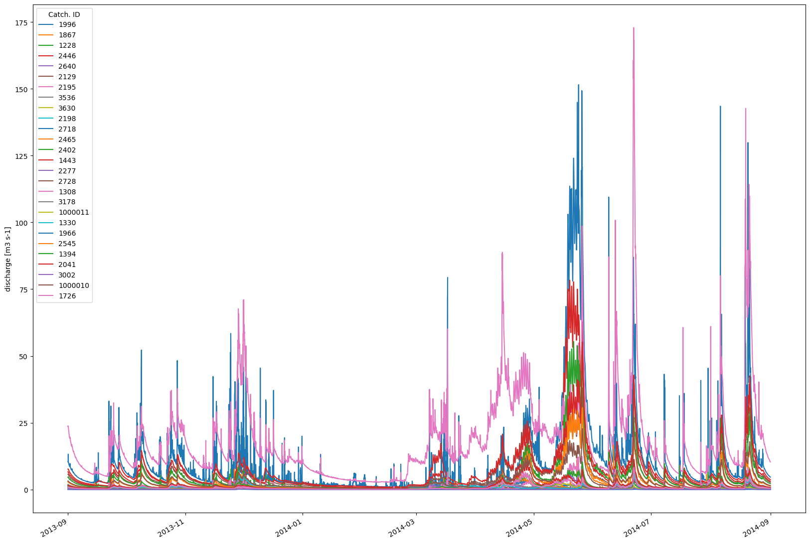
Visualizing the discharge for each [sub-]catchment
Recall that we earlier referred to the importance of understanding the region_model. You’ll see now that this is where information from the simulation is actually contained, and that the simulator object is more or less a convenience wrapper.
# Here we are going to extact data from the simulator object.
# let's work directly with the `region_model`
region_model = simulator.region_model

print(region_model.catchment_ids)
Output:
[   1996    1867    1228    2446    2640    2129    2195    3536    3630
    2198    2718    2465    2402    1443    2277    2728    1308    3178
    1000011    1330    1966    2545    1394    2041    3002 1000010    1726]
We see here that each sub-catchment in our simulation is associated with a unique ID. These are user defined IDs. In the case of the nea-nidelva simulation, they are taken from the GIS database used to create the example configuration files.
To get data out of the region_model you need to specify which catchments you are interested in evaluating. In the following example we are going to extract the data for each catchment and make a simple plot.
Note that Shyft uses many specialized C++ types. Many of these have methods to convert to the more familiar numpy objects. An example may be the discharge timeseries for a catchment.
q_1228_ts = simulator.region_model.statistics.discharge([1228])
q_1228_np = simulator.region_model.statistics.discharge([1228]).values
print(type(q_1228_ts))
print(type(q_1228_np))
Look at the discharge timeseries
As mentioned above, Shyft has it’s own Timeseries class. This class is quite powerful, and the api-timeseries notebook shows more of the functionality. For now, let’s look at some key aspects, and how to create a quick plot of the individual catchment discharge.
# We can make a quick plot of the data of each sub-catchment
fig, ax = plt.subplots(figsize=(20,15))

timestamps = [region_model.time_axis.time(i) for i in range(0, region_model.time_axis.n)]
ts_timestamps = [dt.datetime.utcfromtimestamp(p.seconds) for p in timestamps]

# plot each catchment discharge in the catchment_ids
for i,cid in enumerate(region_model.catchment_ids):
    # a ts.time_axis can be enumerated to it's UtcPeriod,
    # that will have a .start and .end of type utctimestamp
    # to use matplotlib support for datetime-axis, we convert it to datetime (as above)

    data = region_model.statistics.discharge([int(cid)]).values

    ax.plot(ts_timestamps,data, label = "{}".format(region_model.catchment_ids[i]))

fig.autofmt_xdate()
ax.legend(title="Catch. ID")
ax.set_ylabel("discharge [m3 s-1]")

Visualizing the distributed catchment data
An important, but difficult concept, to remember when working with Shyft, is that internally there is no ‘grid’ to speak of. The simulation is vectorized, and each ‘cell’ represents a spatial area with it’s own area and geolocation information. Therefore, we cannot just load a datacube of data, as some may be familiar with.
Visualization of this data is a bit more complex, because each individual cell is in practice an individual polygon. Depending on how the data has been configured for Shyft (see region_model), the cells may, in fact, be simple squares or more complex shapes. For the visualization below, we simply treat them as uniform size, and plot them with the scatter function in matplotlib.
Extract data for individual simulation cells
We’ll start by looking at values of individual cells, rather than at the catchment level. Since Shyft does not have an underlying ‘raster’ model, you need to fetch all cells directly from the underlying region_model.
cells = region_model.get_cells()

# Once we have the cells, we can get their coordinate information
# and fetch the x- and y-location of the cells
x = np.array([cell.geo.mid_point().x for cell in cells])
y = np.array([cell.geo.mid_point().y for cell in cells])
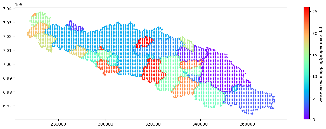
We also will need to get a ‘z’ value to make things interesting. Since this is the first time we’ve visualized our catchment, let’s make a map of the sub-catchments. To do this, the first thing we need to do is get the membership of each cell. That is, to which catchment does it below. We do this by extracting the catchment_id of each cell – and this is what we’ll map. The result will be a map of the sub-catchments.
Recall from above we extracted the catchment_id_map from the region_model:
# mapping of internal catch ID to catchment
catchment_id_map = simulator.region_model.catchment_id_map

# let's create the mapping of catchment_id to an integer:
catchment_ids = region_model.catchment_ids
cid_z_map = dict([ (catchment_ids[i],i) for i in range(len(catchment_ids))])

# then create an array the same length as our 'x' and 'y', which holds the
# integer value that we'll use for the 'z' value
catch_ids = np.array([cid_z_map[cell.geo.catchment_id()] for cell in cells])

# and make a quick catchment map...
# using a scatter plot of the cells
fig, ax = plt.subplots(figsize=(15,5))
cm = plt.cm.get_cmap('rainbow')
plot = ax.scatter(x, y, c=catch_ids, marker='.', s=40, lw=0, cmap=cm)
plt.colorbar(plot).set_label('zero-based mapping(proper map tbd)')

Visualing the Snow Cover Area of all cells for a certain point in time
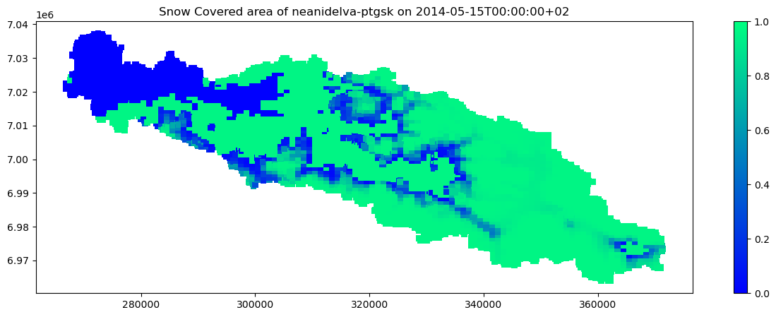
Here we’ll do some more work to look at a snapshot value of data in each of the cells. This example is collecting the response variable (here the Snow Cover Area (SCA)) for each of the cells for a certain point of time.
The “response collector” is another concept within Shyft that is important keep in mind. We don’t collect and store responses for every variable, in order to keep the simulation memory use lean. Therefore, depending on your application, it may be required to explicitly enable this. The relevant code is found in region_model.h in the C++ core source code.
For the ConfigSimulator class, which we used to instantiate the simulator, a standard collector is used that will provide access to the most relevant variables.
For a model run during calibration, we are use a collector that just does the required minimum for the calibration. And, it is still configurable: we can turn on/off the snow-collection, so if we don’t calibrate for snow, they are not collected. More on calibration is shown in the tutorial: Calibration with Shyft
The state collector used for the ‘highspeed’ calibration models (C++), is a null-collector, so no memory allocated, and no cpu-time used.
#first, set a date: year, month, day, (hour of day if hourly time step)
oslo = sts.Calendar('Europe/Oslo') # specifying input calendar in Oslo tz-id
time_x = oslo.time(2014,5,15)  # the oslo calendar(incl dst) converts calendar coordinates Y,M,D.. to its utc-time

# we need to get the index of the time_axis for the time
try:
    idx = simulator.region_model.time_axis.index_of(time_x) # index of time x on time-axis
except:
    print("Date out of range, setting index to 0")
    idx = 0

# fetching SCA (the response variable is named "snow_sca")
# You can use tab-completion to explore the `rc`, short for "response collector"
# object of the cell, to see further response variables available.
# specifying empty list [] indicates all catchments, otherwise pass catchment_id
sca = simulator.region_model.gamma_snow_response.sca([],idx)
Let’s take a closer look at this…
simulator.region_model.time_axis.index_of(time_x)
Simply provided an index value that we can use to index the cells for the time we’re interested in looking at.
Next we use:
simulator.region_model.gamma_snow_response
What is this? This is a collector from the simulation. In this case, for the gamma_snow routine. It contains a convenient method to access the response variables from the simulation on a per catchment level. Each response variable (outflow, sca, swe) can be called with two arguments. The first a list of the catchments, and the second an index to the time, as shown above. Note, this will return the values for each cell in the sub-catchment. Maybe one is only interested in the total outflow or total swe for the region. In this case you can use: .outflow_value which will return a single value.
There is also a response collector for the state variables: .gamma_snow_state.
Explore both of these further with tab completion or help. As well as the full region_model to see what other algorithm collectors are available as this example is configured.
# for attr in dir(simulator.region_model):
#     if attr[0] is not '_': #ignore privates
#         print(attr)
# # and don't forget:
# help(simulator.region_model.gamma_snow_state)
We are now ready to explore some of the variables from the simulation. We’ll continue on with SCA.
# We can make a simple scatter plot again for quick visualization
fig, ax = plt.subplots(figsize=(15,5))
cm = plt.cm.get_cmap('winter')
plot = ax.scatter(x, y, c=sca,
                vmin=0, vmax=1,
                marker='s', s=40, lw=0,
                cmap=cm)
plt.colorbar(plot)
plt.title('Snow Covered area of {0} on {1}'.format(cfg.region_model_id, oslo.to_string(time_x)))

A note about the geometry of the region
Again, keep in mind that while we have created a variable that contains the values for sca in each cell, this is only an iterable object. The only reason we know where each value is located is because we have corresponding x and y values for each cell. It is not an array.
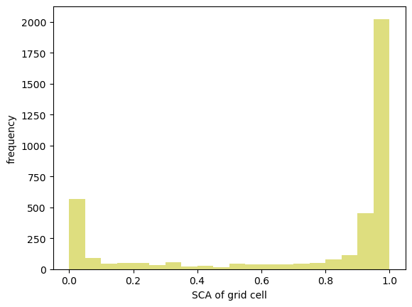
We can calculate some statistics directly out of sca:
# look at the catchment-wide average:
nea_avg_sca = np.average(sca)
print("Average SCA for Nea Nidelva: {0}".format(nea_avg_sca)) # Average SCA for Nea Nidelva: 0.7173656289377036

# And let's compute histogram of the snow covered area as well
fig, ax = plt.subplots()
ax.hist(sca, bins=20, range=(0,1), color='y', alpha=0.5)
ax.set_xlabel("SCA of grid cell")
ax.set_ylabel("frequency")
