Penman-Monteith Sensitivity

Setup environment for tutorials

The purpose of this notebook is to show some simple sensitivity analysis of Penman-Monteith equation shyft implementation.

The function to run the 1-hour time-step Penman-Monteith equation from shyft

We can choose between FPM or SPM methods

import numpy as np
from matplotlib import pyplot as plt
import math
from shyft.time_series import (Calendar,deltahours,TimeSeries,TimeAxis,DoubleVector,point_interpretation_policy)
import shyft.hydrology as api

def run_pm(ws_Th, ws_eah, ws_Rsh, ws_windspeedh,ws_rhh, rnet,
       height_veg=0.12,dt=1, n=30,rl = 144.0,height_ws = 3,
       height_t = 1.68, elevation = 1462.4, method='asce-ewri'):
    """Run Penman-Monteith evapotranspiration model from Shyft"""


    utc = Calendar()

    c_MJm2d2Wm2 = 0.086400
    c_MJm2h2Wm2 = 0.0036

    # n = 30 # nr of time steps: 1 year, daily data
    t_starth = utc.time(2000, 7, 1,16,0,0,0) # starting at 1-07-2000
    step = deltahours(dt)


    # Let's now create Shyft time series from the supplied lists of precipitation and temperature.
    # First, we need a time axis, which is defined by a starting time, a time step and the number of time steps.
    ta = TimeAxis(t_starth, step, n) # days

    # First, we convert the lists to shyft internal vectors of double values:
    temph_dv = DoubleVector.from_numpy(ws_Th)
    eah_dv = DoubleVector.from_numpy(ws_eah)
    rsh_dv = DoubleVector.from_numpy(ws_Rsh)
    windspeedh_dv = DoubleVector.from_numpy(ws_windspeedh)

    rhh_dv = DoubleVector.from_numpy(ws_rhh)

    # Finally, we create shyft time-series as follows:
    # (Note: This step is not necessarily required to run the single methods.
    #  We could also just work with the double vector objects and the time axis)
    instant = point_interpretation_policy.POINT_INSTANT_VALUE
    average = point_interpretation_policy.POINT_AVERAGE_VALUE

    temph_ts = TimeSeries(ta, temph_dv, point_fx=instant)
    eah_ts = TimeSeries(ta, eah_dv, point_fx=instant)
    rsh_ts = TimeSeries(ta, rsh_dv, point_fx=instant)
    windspeedh_ts = TimeSeries(ta, windspeedh_dv, point_fx=instant)

    #recalculated inputs:
    rhh_ts = TimeSeries(ta, rhh_dv, point_fx=instant)

    if method=='asce-ewri':
        full_model = False
    else:
        full_model = True

    pmph = api.PenmanMonteithParameter(height_veg,height_ws,height_t, rl, full_model)
    pmch = api.PenmanMonteithCalculator(pmph)
    pmrh = api.PenmanMonteithResponse()

    #PriestleyTaylor
    ptp = api.PriestleyTaylorParameter(0.2,1.26)
    ptc = api.PriestleyTaylorCalculator(0.2, 1.26)
    ptr = api.PriestleyTaylorResponse

    ET_ref_sim_h= []

    for i in range(n-1):
        pmch.reference_evapotranspiration(pmrh, step,rnet[i], temph_ts.v[i],temph_ts.v[i],
                                                    rhh_ts.v[i], elevation, windspeedh_ts.v[i])
        ET_ref_sim_h.append(pmrh.et_ref)

    return ET_ref_sim_h

So this is our main code to study sensitivity

So here is some sensitivity analysis. First of all, some basic imports and station data (the notebook is nased on ASCE-EWRI Appendix C data).

# Single method test based on ASCE-EWRI Appendix C, hourly time-step
latitude = 40.41
longitude = 104.78
elevation = 1462.4
height_ws = 3 # height of anemometer
height_t = 1.68 # height of air temperature and rhumidity measurements
surface_type = "irrigated grass"
height_veg = 0.12 #vegetation height
# height_veg = 0.5 #tall
atm_pres_mean = 85.17  # [kPa]
psychrom_const = 0.0566
windspeed_adj = 0.921

# Data from weather station
ws_Th = [30.9, 31.2, 29.1, 28.3, 26.0, 22.9, 20.1, 19.9, 18.4, 16.5, 15.4, 15.5, 13.5, 13.2, 16.2, 20.0, 22.9, 26.4,
        28.2, 29.8, 30.9, 31.8, 32.5, 32.9, 32.4, 30.2, 30.6, 28.3, 25.9, 23.9]
ws_eah = [1.09, 1.15, 1.21, 1.21, 1.13, 1.20, 1.35, 1.35, 1.32, 1.26, 1.34, 1.31, 1.26, 1.24, 1.31, 1.36, 1.39, 1.25,
        1.17, 1.03, 1.02, 0.98, 0.87, 0.86, 0.93, 1.14, 1.27, 1.27, 1.17, 1.20]
ws_Rsh = [2.24, 1.65, 0.34, 0.32, 0.08, 0.0, 0.0, 0.0, 0.0, 0.0, 0.0, 0.0, 0.0, 0.03, 0.46, 1.09, 1.74, 2.34, 2.84,
        3.25, 3.21, 3.34, 2.96, 2.25, 1.35, 0.88, 0.79, 0.27, 0.03, 0.0]
ws_windspeedh = [4.07, 3.58, 1.15, 3.04, 2.21, 1.04, 0.58, 0.95, 0.30, 0.50, 1.00, 0.68, 0.69, 0.29, 1.24, 1.28, 0.88,
                0.72, 1.52, 1.97, 2.07, 2.76, 2.90, 3.10, 2.77, 3.41, 2.78, 2.95, 3.27, 2.86]

def rhh_fun(Th, eah):
    rhh = []
    for i in range(len(Th)):
        svp_tmean = 0.6108 * math.exp(17.27 * Th[i] / (Th[i] + 237.3))
        rhh.append(eah[i] * 100 / svp_tmean)
    return rhh

ws_rhh = rhh_fun(ws_Th, ws_eah)

Rnet_orig_h = [1.441, 1.009, 0.244, 0.229, 0.044, -0.016, -0.015, -0.015, -0.015, -0.014, -0.014, -0.014, -0.014, 0.009,
            0.340, 0.616, 1.096, 1.524, 1.888, 2.171, 2.164, 2.239, 1.964, 1.485, 0.905, 0.593, 0.461, 0.065, -0.12]

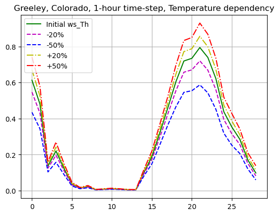
Temperature sensitivity

Temperature impact: we will use original station data as a basis and add/substitude 20 and 50 percent.

# Temperature impact
ws_Th_p20 = []
ws_Th_m20 = []
ws_Th_p50 = []
ws_Th_m50 = []
for t in ws_Th:
    ws_Th_p20.append(t + t * 0.2)
    ws_Th_m20.append(t - t * 0.2)
    ws_Th_p50.append(t + t * 0.5)
    ws_Th_m50.append(t - t * 0.5)

We will use the SPM model here.

result = run_pm(ws_Th, ws_eah, ws_Rsh, ws_windspeedh,ws_rhh, Rnet_orig_h)
plt.plot(result,'g',label='Initial ws_Th')
result2 = run_pm(ws_Th_m20, ws_eah, ws_Rsh, ws_windspeedh,ws_rhh,Rnet_orig_h)
plt.plot(result2,'m--',label='-20%')
result4 = run_pm(ws_Th_m50, ws_eah, ws_Rsh, ws_windspeedh,ws_rhh, Rnet_orig_h)
plt.plot(result4,'b--',label='-50%')
result1 = run_pm(ws_Th_p20, ws_eah, ws_Rsh, ws_windspeedh,ws_rhh, Rnet_orig_h)
plt.plot(result1,'y-.',label='+20%')
result3 = run_pm(ws_Th_p50, ws_eah, ws_Rsh, ws_windspeedh,ws_rhh, Rnet_orig_h)
plt.plot(result3,'r-.',label='+50%')

plt.legend(loc="upper left")

plt.title("Greeley, Colorado, 1-hour time-step, Temperature dependency")
plt.grid(True)
plt.show()

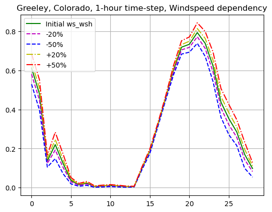
Windspeed sensitivity

#windspeed impact
ws_wsh_p20 = []
ws_wsh_m20 = []
ws_wsh_p50 = []
ws_wsh_m50 = []
for ws in ws_windspeedh:
    ws_wsh_p20.append(ws + ws * 0.2)
    ws_wsh_m20.append(ws - ws * 0.2)
    ws_wsh_p50.append(ws + ws * 0.5)
    ws_wsh_m50.append(ws - ws * 0.5)

result = run_pm(ws_Th, ws_eah, ws_Rsh, ws_windspeedh,ws_rhh, Rnet_orig_h)
plt.plot(result,'g',label='Initial ws_wsh')
result2 = run_pm(ws_Th, ws_eah, ws_Rsh, ws_wsh_m20,ws_rhh, Rnet_orig_h)
plt.plot(result2,'m--',label='-20%')
result4 = run_pm(ws_Th, ws_eah, ws_Rsh, ws_wsh_m50,ws_rhh, Rnet_orig_h)
plt.plot(result4,'b--',label='-50%')
result1 = run_pm(ws_Th, ws_eah, ws_Rsh, ws_wsh_p20,ws_rhh, Rnet_orig_h)
plt.plot(result1,'y-.',label='+20%')
result3 = run_pm(ws_Th, ws_eah, ws_Rsh, ws_wsh_p50,ws_rhh, Rnet_orig_h)
plt.plot(result3,'r-.',label='+50%')

plt.legend(loc="upper left")

plt.title("Greeley, Colorado, 1-hour time-step, Windspeed dependency")
plt.grid(True)
plt.show()

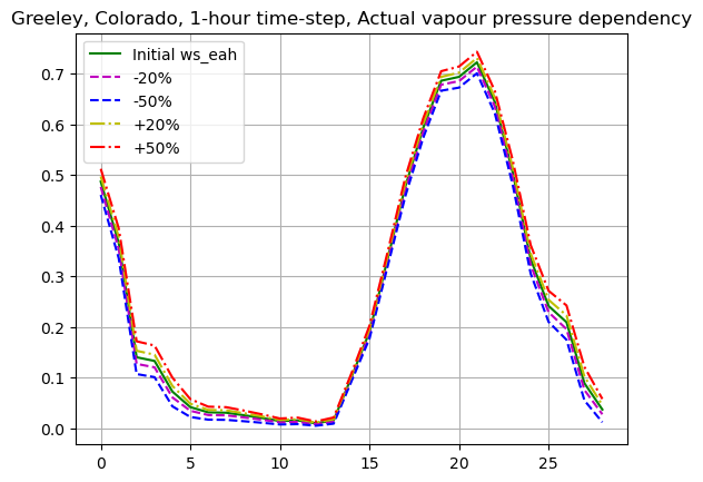
Actual vapor pressure/relative humidity

# actual vapour pressure impact
ws_eah_p20 = []
ws_eah_m20 = []
ws_eah_p50 = []
ws_eah_m50 = []
for ea in ws_eah:
    ws_eah_p20.append(ea + ea * 0.2)
    ws_eah_m20.append(ea - ea * 0.2)
    ws_eah_p50.append(ea + ea * 0.5)
    ws_eah_m50.append(ea - ea * 0.5)

ws_rhh = rhh_fun(ws_Th, ws_eah)
ws_rhh_p20 = rhh_fun(ws_Th, ws_eah_p20)
ws_rhh_m20 = rhh_fun(ws_Th, ws_eah_m20)
ws_rhh_p50 = rhh_fun(ws_Th, ws_eah_p50)
ws_rhh_m50 = rhh_fun(ws_Th, ws_eah_m50)

result = run_pm(ws_Th, ws_eah, ws_Rsh, ws_eah,ws_rhh, Rnet_orig_h)
plt.plot(result,'g',label='Initial ws_eah')
result2 = run_pm(ws_Th, ws_eah, ws_Rsh, ws_eah_m20,ws_rhh, Rnet_orig_h)
plt.plot(result2,'m--',label='-20%')
result4 = run_pm(ws_Th, ws_eah, ws_Rsh, ws_eah_m50,ws_rhh, Rnet_orig_h)
plt.plot(result4,'b--',label='-50%')
result1 = run_pm(ws_Th, ws_eah, ws_Rsh, ws_eah_p20,ws_rhh, Rnet_orig_h)
plt.plot(result1,'y-.',label='+20%')
result3 = run_pm(ws_Th, ws_eah, ws_Rsh, ws_eah_p50,ws_rhh, Rnet_orig_h)
plt.plot(result3,'r-.',label='+50%')

plt.legend(loc="upper left")

plt.title("Greeley, Colorado, 1-hour time-step, Actual vapour pressure dependency")
plt.grid(True)
plt.show()

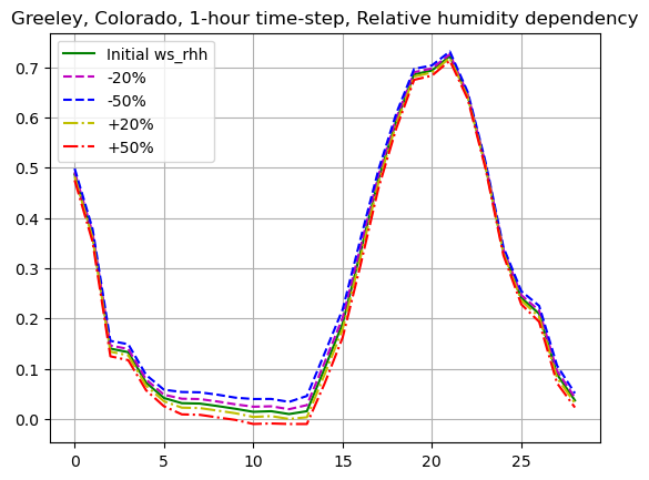
# relative humidity impact
ws_rhh_p20 = []
ws_rhh_m20 = []
ws_rhh_p50 = []
ws_rhh_m50 = []
for rh in ws_rhh:
    ws_rhh_p20.append(rh + rh * 0.2)
    ws_rhh_m20.append(rh - rh * 0.2)
    ws_rhh_p50.append(rh + rh * 0.5)
    ws_rhh_m50.append(rh - rh * 0.5)

result = run_pm(ws_Th, ws_eah, ws_Rsh, ws_eah,ws_rhh, Rnet_orig_h)
plt.plot(result,'g',label='Initial ws_rhh')
result2 = run_pm(ws_Th, ws_eah, ws_Rsh, ws_eah,ws_rhh_m20, Rnet_orig_h)
plt.plot(result2,'m--',label='-20%')
result4 = run_pm(ws_Th, ws_eah, ws_Rsh, ws_eah,ws_rhh_m50, Rnet_orig_h)
plt.plot(result4,'b--',label='-50%')
result1 = run_pm(ws_Th, ws_eah, ws_Rsh, ws_eah,ws_rhh_p20, Rnet_orig_h)
plt.plot(result1,'y-.',label='+20%')
result3 = run_pm(ws_Th, ws_eah, ws_Rsh, ws_eah,ws_rhh_p50, Rnet_orig_h)
plt.plot(result3,'r-.',label='+50%')

plt.legend(loc="upper left")

plt.title("Greeley, Colorado, 1-hour time-step, Relative humidity dependency")
plt.grid(True)
plt.show()

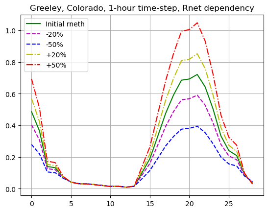
Rnet sensitivity

# rnet impact
rneth_p20 = []
rneth_m20 = []
rneth_p50 = []
rneth_m50 = []
for rnet in Rnet_orig_h:
    rneth_p20.append(rnet + rnet * 0.2)
    rneth_m20.append(rnet - rnet * 0.2)
    rneth_p50.append(rnet + rnet * 0.5)
    rneth_m50.append(rnet - rnet * 0.5)

result = run_pm(ws_Th, ws_eah, ws_Rsh, ws_eah,ws_rhh, Rnet_orig_h)
plt.plot(result,'g',label='Initial rneth')
result2 = run_pm(ws_Th, ws_eah, ws_Rsh, ws_eah,ws_rhh, rneth_m20)
plt.plot(result2,'m--',label='-20%')
result4 = run_pm(ws_Th, ws_eah, ws_Rsh, ws_eah,ws_rhh, rneth_m50)
plt.plot(result4,'b--',label='-50%')
result1 = run_pm(ws_Th, ws_eah, ws_Rsh, ws_eah,ws_rhh, rneth_p20)
plt.plot(result1,'y-.',label='+20%')
result3 = run_pm(ws_Th, ws_eah, ws_Rsh, ws_eah,ws_rhh, rneth_p50)
plt.plot(result3,'r-.',label='+50%')

plt.legend(loc="upper left")

plt.title("Greeley, Colorado, 1-hour time-step, Rnet dependency")
plt.grid(True)
plt.show()

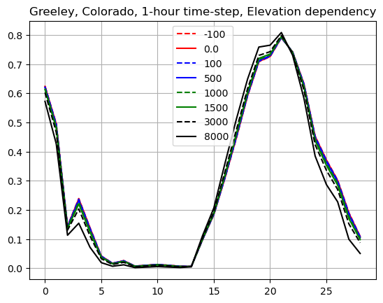
Elevation

# elevation

dt = 1
n = 30
lai = 2.0
rl = 144
elevation_array = [-100, 0.0, 100, 500, 1000, 1500, 3000, 8000]
colors = ('r--','r', 'b--','b','g--','g','k--','k')
i = 0
for elevation in elevation_array:
    result = run_pm(ws_Th, ws_eah, ws_Rsh, ws_windspeedh,ws_rhh, Rnet_orig_h, height_veg,dt, n,rl,height_ws, height_t, elevation)
    plt.plot(result,colors[i],label=elevation)
    i+=1

plt.legend(loc="upper center")

plt.title("Greeley, Colorado, 1-hour time-step, Elevation dependency")
plt.grid(True)
plt.show()

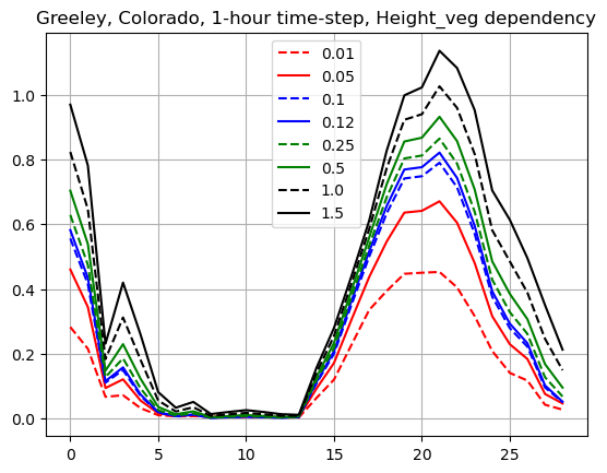
Sensitivity to parameters we will study using FPM

Vegetation height

# height vegetation

dt = 1
n = 30
rl = 72
hveg_array = [0.01, 0.05, 0.1, 0.12, 0.25, 0.5, 1.0, 1.5]
colors = ('r--','r', 'b--','b','g--','g','k--','k','m--','m')
i = 0
for height_veg in hveg_array:
    result = run_pm(ws_Th, ws_eah, ws_Rsh, ws_windspeedh,ws_rhh, Rnet_orig_h, height_veg,dt, n,rl,height_ws, height_t, elevation,'full')
    plt.plot(result,colors[i],label=height_veg)
    i+=1

plt.legend(loc="upper center")

plt.title("Greeley, Colorado, 1-hour time-step, Height_veg dependency")
plt.grid(True)
plt.show()

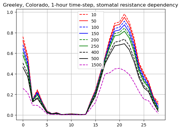
Stomatal resistance

# effective stimatal resistanse

dt = 1
n = 30
rl = 144
height_veg = 0.5
rl_array = [10, 50, 100, 150, 200,250, 400, 500,1500]
colors = ('r--','r', 'b--','b','g--','g','k--','k','m--','m')
i = 0
for rl in rl_array:
    result = run_pm(ws_Th, ws_eah, ws_Rsh, ws_windspeedh,ws_rhh, Rnet_orig_h, height_veg,dt, n,rl,height_ws, height_t, elevation,'full')
    plt.plot(result,colors[i],label=rl)
    i+=1

plt.legend(loc="upper center")

plt.title("Greeley, Colorado, 1-hour time-step, stomatal resistance dependency")
plt.grid(True)
plt.show()

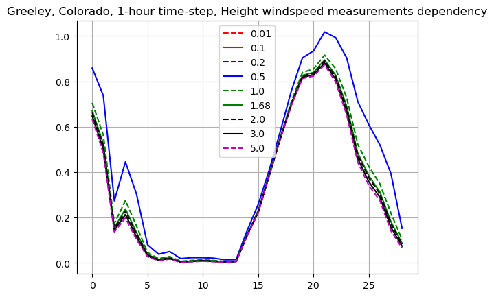
WS measurements height

# ws measurements height
dt = 1
n = 30
lai = 2.0
rl = 144
height_ws_array = [0.01, 0.1, 0.2, 0.5, 1.0, 1.68, 2.0, 3.0, 5.0]
colors = ('r--','r', 'b--','b','g--','g','k--','k','m--','m')
i = 0
for height_ws in height_ws_array:
    result = run_pm(ws_Th, ws_eah, ws_Rsh, ws_windspeedh,ws_rhh, Rnet_orig_h, height_veg,dt, n,rl,height_ws, height_t, elevation,'full')
    plt.plot(result,colors[i],label=height_ws)
    i+=1

plt.legend(loc="upper center")

plt.title("Greeley, Colorado, 1-hour time-step, Height windspeed measurements dependency")
plt.grid(True)
plt.show()

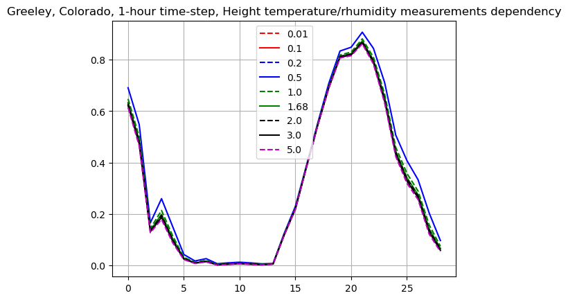
Temperature and humidity measurements height

# t measurements height
dt = 1
n = 30
lai = 2.0
rl = 144
height_t_array = [0.01, 0.1, 0.2, 0.5, 1.0, 1.68, 2.0, 3.0, 5.0]
colors = ('r--','r', 'b--','b','g--','g','k--','k','m--','m')
i = 0
for height_t in height_t_array:
    result = run_pm(ws_Th, ws_eah, ws_Rsh, ws_windspeedh,ws_rhh, Rnet_orig_h, height_veg,dt, n,rl,height_ws, height_t, elevation,'full')
    plt.plot(result,colors[i],label=height_t)
    i+=1

plt.legend(loc="upper center")

plt.title("Greeley, Colorado, 1-hour time-step, Height temperature/rhumidity measurements dependency")
plt.grid(True)
plt.show()